Challenge

Week 5.1 - Mid term project - Solving the steady and unsteady 2D heat conduction problem

HHarikrishnan Muralidharan9 Apr 2024

ASSIGNMENT

AIM: The assignment aims to solve the 2D heat conduction equation using an iterative solver and understand the plots.

TOOLS USED: Matlab Programming

GENERAL THEORY: The 2D transient and 2D steady state heat conduction equations are given below as follows :

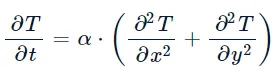....................... (1)

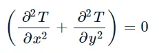.................................(2)

These are partially differential equations that cannot be solved analytically( though it can solved in certain cases where the geometry has high level of symmetry) so we need to use numerical methods to solve these equations. We use a an FDM approch to change this to a numerical equation and we use iterative approches to get the solution.

In this assignment we develop a code to solve the 2D steady state and transient heat conduction equation numerically. We solve using both implicit and explicit methods.

We start by understanding the boundary conditions. So in this , the BCs are given as shown in the figure below :

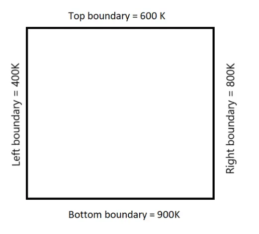
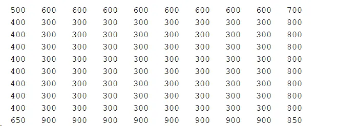
The inner nodal values are 300 K. So when all the temperature values are initialized, you will get something like this :

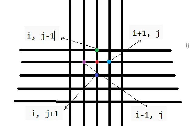
The nodal points can be seen in the figure below. If the present node is i,j :

CODE TRANSIENT 2D IMPLICIT

Theory : The transient 2D heat conduction equation is given by :

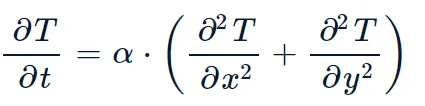
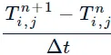
here we have the time marching term and the space term. They are discretized as per given below :

and for the conduction term :

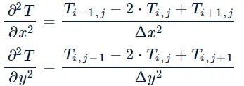
here , we are solving the equation using an implicit method, because of which we use an itreative solvers. So before we discuss the various iterative solvers, we need to understand what implicit method is.

The implicit discretization of the 2d Heat conduction equation involves discretization of the spatial derivatives using central differencing and the temporal derivatives using forward differencing. If the grid points are represented as i,j and Tn(i,j) is the temperature at n th timestep for the i,j, we have the equation

Rearranging this equation , we get

This equation represents a system of linear equations for each grid points which is solved iteratively for the n+1 timesteps. Since this is an implicit method, we use iterative solvers as methods like gauss elimination and other direct methods become computationally expensive. There are mainly three types of iterative solvers we use

Jacobi
Gauss Siedel
SOR(Successive over relaxation)

It will be explained one by one

Jacobi:

The Jacobi method is based on solving for every variable locally with respect to the other variables; one iteration of the method corresponds to solving for every variable once. The resulting method is easy to understand and implement, but convergence is slow.

Gauss Siedel

The Gauss-Seidel method is like the Jacobi method, except that it uses updated values as soon as they are available. In general, if the Jacobi method converges, the Gauss-Seidel method will converge faster than the Jacobi method, though still relatively slowly.

SOR

Successive Overrelaxation (SOR) can be derived from the Gauss-Seidel method by introducing an extrapolation parameter . For the optimal choice of , SOR may converge faster than Gauss-Seidel by an order of magnitude.

Code and explanation:

%CODE FOR TRANSIENT 2D HEAT CONDUCTION -IMPLICIT

clear all 
close all
clc

nx=10;                       %number of nodal points in x direction
ny=10;                       % number of nodal points in y direction
T= 0.15;                     %total time
t_ini=300*ones(nx,ny);       %initial conditions of the temperature
dt=0.0001;                   %time step
alpha=1.4;
nt=T/dt;
x = linspace(0,1,nx);        %distance between 2 nodes in x direction
y = linspace(0,1,ny);        %distance between 2 nodes in y direction

%jacobi(nx,ny,dt, alpha) initial condition

for i=1:nx
    t_ini(1,i)=600;
end
     
for i=1:ny
    t_ini(i,1)=400;
end
       
t_ini(1,1)=500;
     
for i=1:nx
    t_ini(ny,i)=900;
end
     
t_ini(ny,1)=650;
       
for i=1:ny
    t_ini(i,nx)=800;
end
       
t_ini(1,nx)=700;     
t_ini(ny,nx)=850;
       
disp('t_ini after the for loop:');
disp(t_ini);

told= t_ini
       
dx=x(2)-x(1);
dy=y(2)-y(1);

k1=(dt*alpha)/dx^2;
k2=(dt*alpha)/dy^2;

tol=1e-4
itr=0;
choice=input('enter 1. jacobi 2. Gauss Seidel 3. SOR')    


if choice ==1      % Jacobi
cho='jacobi';   
    tic
    for p=1:nt
       error=9e9;
       
       while(error>tol)
            for i=2:nx-1
                for j=2:ny-1
                    term1 = (1+(2*k1)+(2*k2))^-1;
                    term2 = k1*term1;
                    term3 = k2*term1;
                    h = (told(i-1,j)+told(i+1,j));
                    v = (told(i,j+1)+told(i,j-1));
                    t_ini(i,j) = ((told(i,j)*term1)+(h*term2)+(v*term3));
                
                
                end          
            
            end
            error = max(max(abs(t_ini-told)));
            told = t_ini;
            itr = itr+1
       
       end 
   
   end
   time_taken=toc;
end



if choice ==2  % Gauss Siedel
cho='Gauss Siedel'   
    tic
    for p=1:nt
       error=9e9;
       while(error>tol)
            for i=2:nx-1
                for j=2:ny-1
                    term1 = (1+(2*k1)+(2*k2))^-1;
                    term2 = k1*term1;
                    term3 = k2*term1;
                    h = (t_ini(i-1,j)+told(i+1,j));
                    v = (told(i,j+1)+t_ini(i,j-1));
                    t_ini(i,j) = ((told(i,j)*term1)+(h*term2)+(v*term3));
                
                
                end          
            
            end
            error = max(max(abs(t_ini-told)));
            told = t_ini;
            itr = itr+1
       
       end 
   
   end
 time_taken=toc;
end




if choice ==3             %SOR
cho='SOR'
omega=input('enter the value of omega');
tic  
for p=1:nt
       error=9e9;
       while(error>tol)
            for i=2:nx-1
                for j=2:ny-1
                    term1 = (1+(2*k1)+(2*k2))^-1;
                    term2 = k1*term1;
                    term3 = k2*term1;
                    h = (t_ini(i-1,j)+told(i+1,j));
                    v = (told(i,j+1)+t_ini(i,j-1));
                    t_ini(i,j) =((1-omega)*told(i,j)) +(omega)*((told(i,j)*term1)+(h*term2)+(v*term3));
                
                
                end          
            
            end
            error = max(max(abs(t_ini-told)));
            told = t_ini;
            itr = itr+1
       
       end 
   
   end
 time_taken=toc;
end 




 
 [X,Y] = meshgrid(x,y);
 contourf(X,Y,t_ini)
 colormap(jet);
 colorbar
 set(gca,'ydir','reverse')
 
 text1 = sprintf('number of iteration = %d', itr);
 text2= sprintf('time taken =%d',time_taken) 

 title_stre=sprintf(' 2D transient heat conduction equation using %s ', cho)
 title({title_stre,text1,text2})
 grid on
 xlabel('X-Direction');
 ylabel('Y-Direction');

Results and discussion:

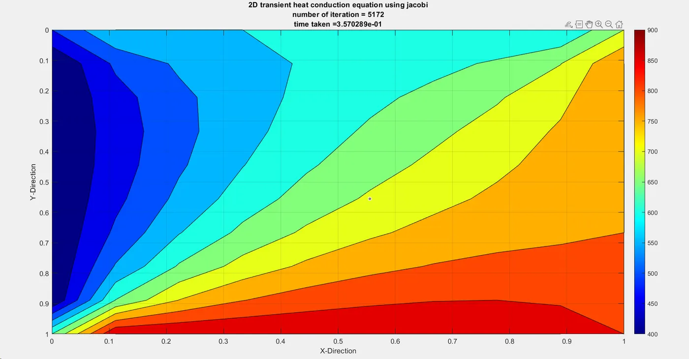
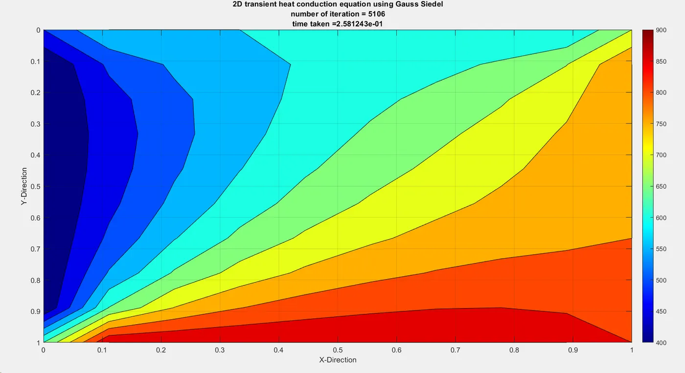
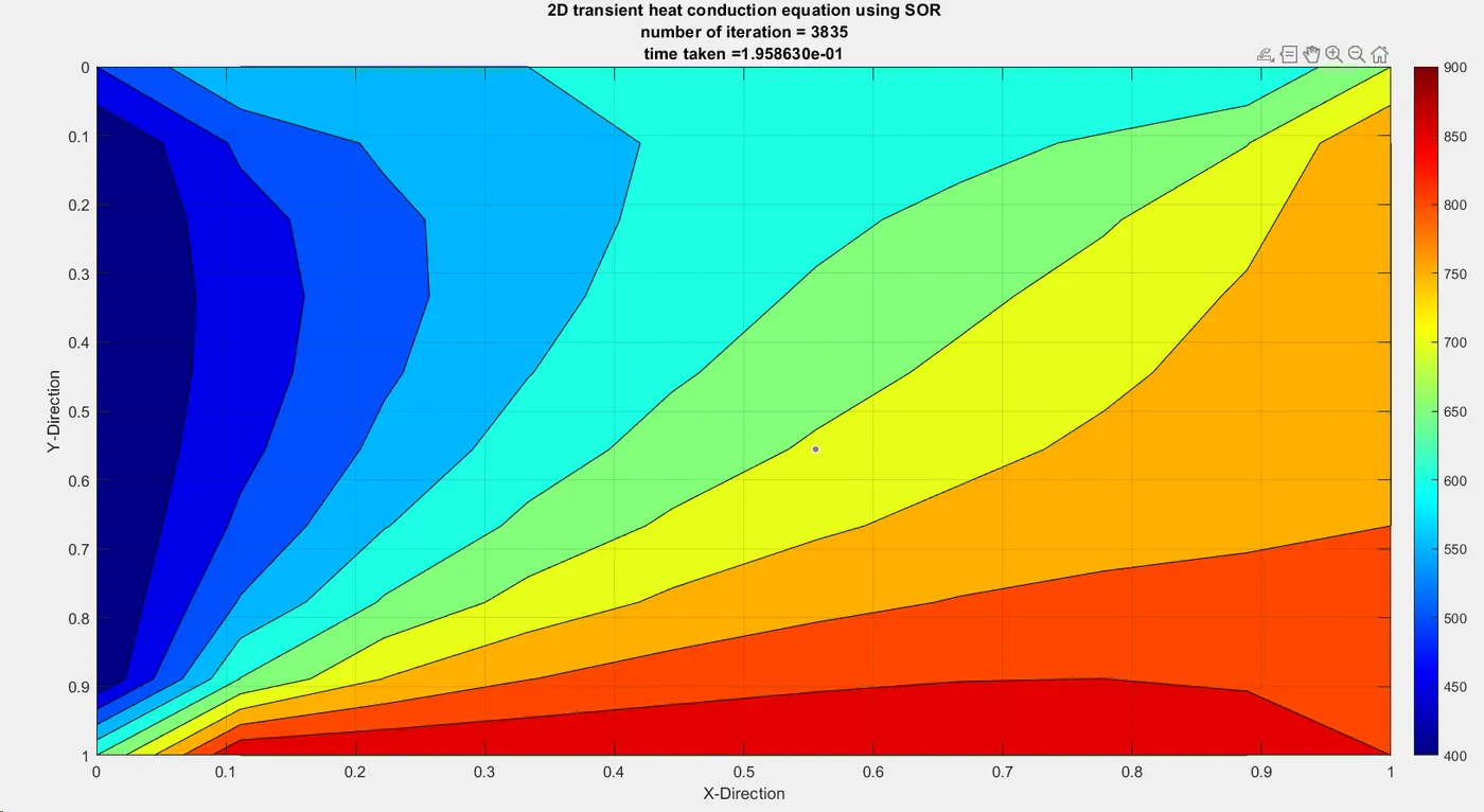
It can be seen that the number of iterations is highest for jacobi followed by Gauss Siedel and SOR respectively.

CODE TRANSIENT 2D EXPLICIT

Theory : For the transient explicit, the equation is given as follows:

here alpha is the thermal diffusivity and delta x and y are the size of the mesh element.

Code and explanation:

% CODE FOR TRANSIENT explicit


clear all 
close all
clc

nx=10;
ny=10;
T= 0.4;
t_ini=300*ones(nx,ny);  %initial conditions
dt=0.001;
alpha=1.4;
nt=1500;
x = linspace(0,1,nx);
y = linspace(0,1,ny);

%jacobi(nx,ny,dt, alpha)

for i=1:nx
    t_ini(1,i)=600;
end
     
for i=1:ny
    t_ini(i,1)=400;
end
       
t_ini(1,1)=500;
     
for i=1:nx
    t_ini(ny,i)=900;
end
     
t_ini(ny,1)=650;
       
for i=1:ny
    t_ini(i,nx)=800;
end
       
t_ini(1,nx)=700;     
t_ini(ny,nx)=850;
       
disp('t_ini after the for loop:');
disp(t_ini);

t_old= t_ini
       
dx=x(2)-x(1);
dy=y(2)-y(1);

k1=(dt*alpha)/dx^2;
k2=(dt*alpha)/dy^2;

tol=1e-4
itr=0;
T=0.04

tic
for g=1:T/dt
    for i=2:ny-1
        for j=2:nx-1
        
            t_ini(i,j)=t_old(i,j)+ (k1* (t_old(i+1,j)-(2*t_old(i,j))+t_old(i-1,j)))+(k2* (t_old(i,j+1)-(2*t_old(i,j))+t_old(i,j-1)))
        
        end
         t_old=t_ini ;
    end



end    
time_taken=toc;

[X,Y] = meshgrid(x,y);
 contourf(X,Y,t_ini)
 colormap(jet);
 colorbar
 set(gca,'ydir','reverse')
 text2= sprintf('time taken =%d',time_taken) 
 title (' Transient Analysis of 2D-heat conduction equation using explicit scheme',text2);
 
 grid on
 xlabel('X-Direction');
 ylabel('Y-Direction');

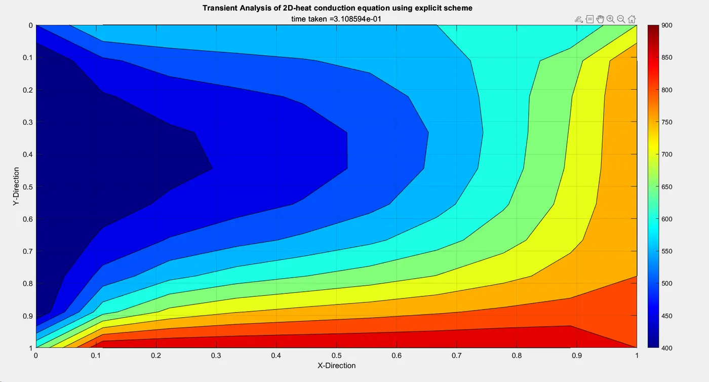
Results and discussion:

CODE STEADY STATE 2D IMPLICIT

Theory :

The equation for the steady state 2D heat conduction is given below :

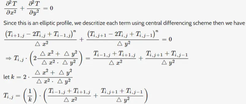
Here we use an iterative process to solve. We use Jacobi, gauss siedel, SOR. The equations are given below

Jacobi : Uses the values in the previous iteration

Gauss Siedel : Uses the recently updated values

SOR : uses a parameter omega to accelerate the convergence

Code and explanation:

% CODE FOR Steady state both implicit 


clear all 
close all
clc

nx=10;
ny=10;
T= 0.4;
t_ini=300*ones(nx,ny);  %initial conditions
dt=0.001;
alpha=1.4;
nt=1500;
x = linspace(0,1,nx);
y = linspace(0,1,ny);

%jacobi(nx,ny,dt, alpha)

for i=1:nx
    t_ini(1,i)=600;
end
     
for i=1:ny
    t_ini(i,1)=400;
end
       
t_ini(1,1)=500;
     
for i=1:nx
    t_ini(ny,i)=900;
end
     
t_ini(ny,1)=650;
       
for i=1:ny
    t_ini(i,nx)=800;
end
       
t_ini(1,nx)=700;     
t_ini(ny,nx)=850;
       
disp('t_ini after the for loop:');
disp(t_ini);

told= t_ini
       
dx=x(2)-x(1);
dy=y(2)-y(1);

k1=(dt*alpha)/dx^2;
k2=(dt*alpha)/dy^2;
 error=9e9;
tol=1e-10
omega=1.4;
T=0.04
k = 2*(dx^2+dy^2)/(dx^2*dy^2);

method = input('Iterative method = '); %iterative method selection

%JACOBI ITERATIVE METHOD

if (method==1)
cho='jacobi'; 
    tic;
    itr=0;
    while(error>tol)
        for i = 2:(nx-1)
            for j = 2:(ny-1)
                 t_ini(i,j)=(((told(i-1,j)+told(i+1,j))/dx^2) +((told(i,j+1)+told(i,j-1))/dy^2))/k;
                
            end
        end
        error = max(max(abs(t_ini-told)));
        told = t_ini;
        itr = itr+1;
        time_taken = toc;
    end
end

 
if (method==2)
cho='Gauss Siedel' 

tic;
    itr=0;
    while(error>tol)
        for i = 2:(nx-1)
            for j = 2:(ny-1)
                 t_ini(i,j)=(((t_ini(i-1,j)+told(i+1,j))/dx^2) +((told(i,j+1)+t_ini(i,j-1))/dy^2))/k;
                 %t_ini(i,j)= told(i,j)*(1-omega) + (omega*(((t_ini(i-1,j)+told(i+1,j))/dx^2) +((told(i,j+1)+t_ini(i,j-1))/dy^2))/k)
            end
        end
        error = max(max(abs(t_ini-told)));
        told = t_ini;
        itr = itr+1;
        time_taken = toc;
    end
end

%  
if (method==3)
omega=input("enter relaxation factor")
cho='SOR' 
    tic;
    itr=0;
    while(error>tol)
        for i = 2:(nx-1)
            for j = 2:(ny-1)
                 %t_ini(i,j)=(((t_ini(i-1,j)+told(i+1,j))/dx^2) +((told(i,j+1)+t_ini(i,j-1))/dy^2))/k;
                 t_ini(i,j)= told(i,j)*(1-omega) + (omega*(((t_ini(i-1,j)+told(i+1,j))/dx^2) +((told(i,j+1)+t_ini(i,j-1))/dy^2))/k)
            end
        end
        error = max(max(abs(t_ini-told)));
        told = t_ini;
        itr = itr+1;
        time_taken = toc;
    end
end


 

 

 [X,Y] = meshgrid(x,y);
 contourf(X,Y,t_ini)
 colormap(jet);
 colorbar
 set(gca,'ydir','reverse')
 
 text1 = sprintf('number of iteration = %d', itr);
 text2= sprintf('time taken =%d',time_taken) 

 title_stre=sprintf(' 2D transient heat conduction equation using %s ', cho)
 title({title_stre,text1,text2})
 grid on
 xlabel('X-Direction');
 ylabel('Y-Direction');

Results and discussion:

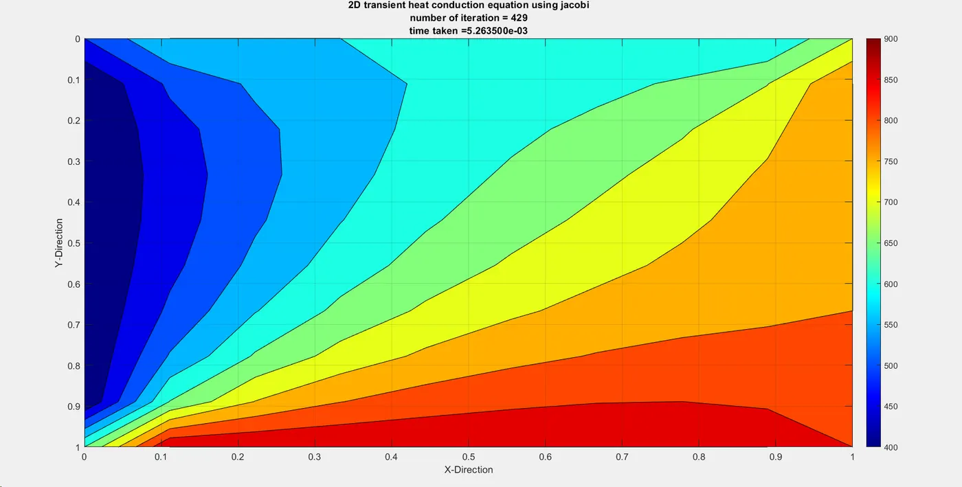
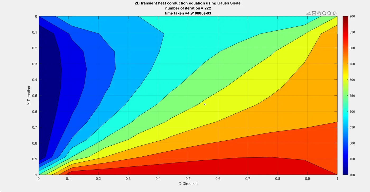
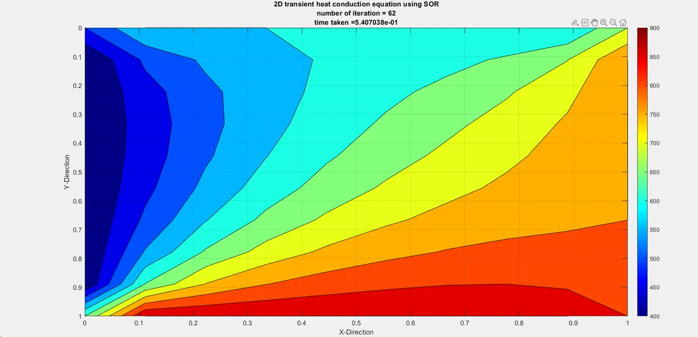
It follows the same trend. Higher number of iterations for Jacobi, followed by Gauss Siedel and SOR respectively.

Week 5.1 - Mid term project - Solving the steady and unsteady 2D heat conduction problem

Ship work like this
in your own course.

Talk to a career counsellor

Ship work like thisin your own course.

Talk to a career counsellor

Ship work like this
in your own course.