Week 5.1 - Mid term project - Solving the steady and unsteady 2D heat conduction problem

AIM : To solve the steady and unsteady state of heat conduction equation.

OBJECTIVE :

Steady state analysis & Transient State Analysis

Solving the 2D heat conduction equation by using the point iterative techniques. The Boundary conditions for the problem are as follows;

• Top Boundary = 600 K
• Bottom Boundary = 900 K
• Left Boundary = 400 K
• Right Boundary = 800 K

implement the following methods for solving implicit equations.

1. Jacobi
2. Gauss-seidel
3. Successive over-relaxation
4. absolute error criteria is 1e-4

PROCEDURE :

DISCRETIZATION : Divide the 2d domain into a grid by selecting the number of nodes in the x and y directions. let's assume there are (n+2) nodes in the x-direction and (m+2) nodes in the y-direction, including boundary nodes. each node represents a point in the domain.

INITIALISE THE GIRD : Assign initial temperatures to the nodes.the boundary nodes will have fixed temperatures according to the given boundary conditions.

STEADY STATE : Use iterative techniques (jacobi, gauss-seidel, sor) to solve the discretized equation until the solution converges. the iterative process involves updating the temperature values of the inner nodes based on neighbouring node values.

TRANSIENT [ EXPLICIT ] : For the transient analysis,we will use an explict scheme to track the evolution of the temperature overtime.the finite difference equation for the explict scheme is derivied from the heat conduction equation.iterate overtime steps and update the temperature values of the inner nodes based on neighbouring node values at the previous time step.

TRANSIENT [ IMPLICIT ] : For the implict scheme ,the finite difference equation is rearranged to express the temperature at the current time step in terms of the temperature at the previous time step.set up a system of equations and solve it using iterative technieques [jacobi,gauss-seidel,sor] until the solution converges.

CONVERGENCE CRITERIA : The convergence criteria for both steady & transient analysis is based on the absolute error between consecutive iterations,the iterative process continues until the absolute error falls below a certain threshold [ eg. 1e-4 ].

COMPARING CONVERGENCE RATES : Compare the number of iterations required for convergence between the steady state and transient [ explicit & implicit ] simulattions.

PROGRAM FOR STEADY STATE CONDITION :

clear all
close all
clc

% steady state heat conducrion equation d^2t/dx^2 + d^2t/dy^2=0

nx=10;
ny=10;

T=450*ones(nx,ny);



%k1=aplha*(dt/dx^2)
%fase tempreture
TL= 400;
TR= 800;
TT = 600;
TB= 900;

%BC
T(:,1)=TL;
T(:,ny)=TR;
T(1,:)=TT;
T(nx,:)=TB;
%edge refinement
T(1,1)=(T(2,1)+T(1,2))/2;
T(nx,1)=(T(nx-1,1)+T(nx,2))/2;
T(nx,ny)= (T(nx-1,ny)+T(nx,ny-1))/2;
T(1,ny)=(T(2,ny)+T(1,ny-1))/2;

Told=T;
Tinitial = T;

% iteration process 1. jacobi 2. gs 3. sor
% 1) jacobi method

error = 9e9;
tol = 1e-4;
jac_itel=0

while(error>tol)

    for i=2:nx-1
        for j= 2:ny-1

            T(i,j)= 0.25*(T(i+1,j) + Told(i-1,j)+Told(i,j-1)+Told(i,j+1));
        end
    end

    error= max(max(abs(T-Told)));
    Told=T;
    jac_itel=jac_itel+1;
    figure(1)
    contourf(flipud(T),'ShowText','ON')

    title(sprintf('steady state jacobi iteration=%d',jac_itel))
    pause(0.003)



end



% reinitializing
T=Tinitial;
Told=T;
error=9e9;
gs_iter=0;
% GS method for itteration

while(error>tol)

    for i=2:nx-1
        for j= 2:ny-1

            T(i,j)= 0.25*(T(i+1,j) + T(i-1,j)+T(i,j-1)+Told(i,j+1));
        end
    end

    error= max(max(abs(T-Told)));
    Told=T;
    gs_iter=gs_iter+1;
    figure(2)
    contourf(flipud(T),'ShowText','ON')

    title(sprintf('steady state GS iteration=%d',gs_iter))
    pause(0.003)



end

%reinitialise for SOR
T=Tinitial;
Told=T;
error=9e9;

%SOR iteration

SOR_iter=0;
omega=1.5;

while(error>tol)

    for i=2:nx-1
        for j= 2:ny-1

            TGS(i,j)= 0.25*(T(i+1,j) + T(i-1,j)+T(i,j-1)+Told(i,j+1));
            T(i,j)=(1-omega)*Told(i,j) + omega*TGS(i,j);


        end
    end

    error= max(max(abs(T-Told)));
    Told=T;
    SOR_iter=SOR_iter+1;
    figure(3)
    contourf(flipud(T),'ShowText','ON')

    title(sprintf('steady state SOR iteration=%d',SOR_iter))
    pause(0.003)



end

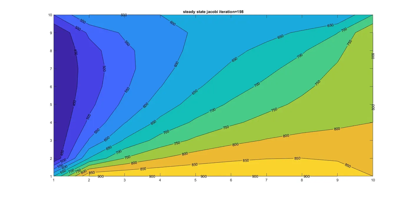
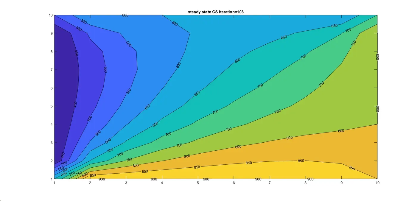
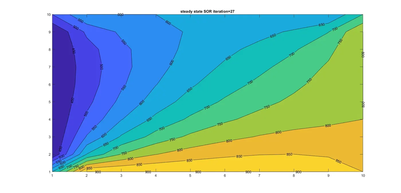
Below graph is for steady 2d state calculation of heat conduction equation, from all graph being same, we can understand the ans. by all 3 methods are same at the end only the no. of iterations it requires varies like in JACOBI method the iteration value is highest, and accordingly SOR method has least iteration.so, the SOR method is faster than compare to other two.

RESULTS :

JACOBI :

GAUSS-SEIDEL :

SOR :

PROGRAM FOR TRANSIENT [UNSTEADY ] STATE CONDITION :

EXPLICIT :

clear all
close all
clc

% steady state heat conducrion equation d^2t/dx^2 + d^2t/dy^2=0

nx=10;
ny=10;

T=450*ones(nx,ny);



%k1=aplha*(dt/dx^2)
%fase tempreture
TL= 400;
TR= 800;
TT = 600;
TB= 900;

%BC
T(:,1)=TL;
T(:,ny)=TR;
T(1,:)=TT;
T(nx,:)=TB;
%edge refinement
T(1,1)=(T(2,1)+T(1,2))/2;
T(nx,1)=(T(nx-1,1)+T(nx,2))/2;
T(nx,ny)= (T(nx-1,ny)+T(nx,ny-1))/2;
T(1,ny)=(T(2,ny)+T(1,ny-1))/2;


Tprev=T;
%timestep
dt=1e-2;
%grid spacing
dx=5e-2;
dy=5e-2;
%thermal diffusity
alpha = 0.015;

k1=alpha*(dt/dx^2);
k2=alpha*(dt/dy^2);

% Time iterative solver


cfl=k1+k2;
conv=9e9;
tol = 1e-4;

time_iter=0;

%time loop
while(conv>tol)

    for i=2:nx-1
        for j= 2:ny-1

            T(i,j)= (1-2*k1-2*k2)*Tprev(i,j)+ k1*(Tprev(i-1,j)+Tprev(i+1,j))+k2*(Tprev(i,j-1)+Tprev(i,j+1));
        end
    end

    conv= max(max(abs(T-Tprev)));
    Tprev=T;
    time_iter=time_iter+1;

    figure(1)
    contourf(flipud(T),'ShowText','ON')

    title(sprintf('Transient explicit time iteration=%d',time_iter))
    pause(0.05)
end

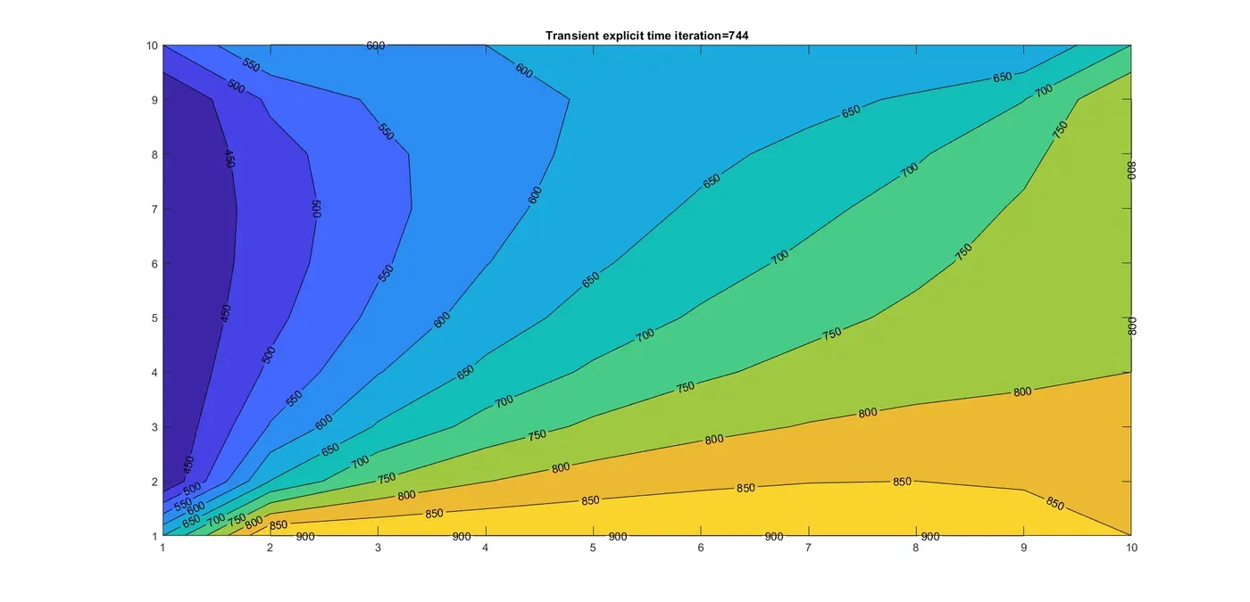
in explicit method only time loop is required, as all adjacent values we use to calculate the next value in next time step is taken from the previous matrix, or previous time step, so, no need of space loop also in implicit method as we have to take values from two matrix the three diff. methods can be use but as in this method all values in rhs are know so no complex calculation, though the output is same, there are some advantages and disadvantages.as in explicit we have to consider clf term which is k1+k2 which should not exceed 0.5 in 2d conduction, otherwise it can blow up the entire solution, so mostly there are some criteria which needs to be taken under consideration for choosing any of these methods

RESULT :

IMPLICIT :

clear all
close all
clc

% steady state heat conducrion equation d^2t/dx^2 + d^2t/dy^2=0

nx=10;
ny=10;

T=450*ones(nx,ny);



%k1=aplha*(dt/dx^2)
%fase tempreture
TL= 400;
TR= 800;
TT = 600;
TB= 900;

%BC
T(:,1)=TL;
T(:,ny)=TR;
T(1,:)=TT;
T(nx,:)=TB;
%edge refinement
T(1,1)=(T(2,1)+T(1,2))/2;
T(nx,1)=(T(nx-1,1)+T(nx,2))/2;
T(nx,ny)= (T(nx-1,ny)+T(nx,ny-1))/2;
T(1,ny)=(T(2,ny)+T(1,ny-1))/2;

Told=T;
Tinitial = T;
Tprev=T;
%timestep
dt=1e-2;
%grid spacing
dx=1e-2;
dy=1e-2;
%thermal diffusity
alpha = 0.015;

k1=alpha*(dt/dx^2);
k2=alpha*(dt/dy^2);

% iteration process 1. jacobi 2. gs 3. sor
% 1) jacobi method

error = 9e9;
conv=9e9;
tol = 1e-4;
jac_itel=0;
Jac_time_iter=0;

%time loop
while(conv>tol)
    %space loop
    while(error>tol)

        for i=2:nx-1
            for j= 2:ny-1

                T(i,j)= (1+2*k1+2*k2)^-1*(Tprev(i,j)+ k1*(Told(i-1,j)+Told(i+1,j))+k2*(Told(i,j-1)+Told(i,j+1)));
            end
        end

        error= max(max(abs(T-Told)));
        Told=T;
        jac_itel=jac_itel+1;
        figure(1)
        contourf(flipud(T),'ShowText','ON')

        title(sprintf('Transient imlicit jacobi iteration=%d \nTime iterations=%d',jac_itel,Jac_time_iter))
        pause(0.003)

    end
    conv= max(max(abs(T-Tprev)));
    Tprev=T;
    Jac_time_iter=Jac_time_iter+1;
    error=9e9;


end




% reinitializing
T=Tinitial;
Told=T;
error=9e9;
gs_iter=0;
gs_time=0;
conv=9e9;
Tprev=T;
% GS method for itteration

%time loop
while(conv>tol)
    %space loop
    while(error>tol)

        for i=2:nx-1
            for j= 2:ny-1

                T(i,j)= (1+2*k1+2*k2)^-1*(Tprev(i,j)+ k1*(T(i-1,j)+Told(i+1,j))+k2*(T(i,j-1)+Told(i,j+1)));
            end
        end

        error= max(max(abs(T-Told)));
        Told=T;
        gs_iter=gs_iter+1;
        figure(2)
        contourf(flipud(T),'ShowText','ON')

        title(sprintf('Transient imlicit gs iteration=%d \nTime iterations=%d',gs_iter,gs_time))
        pause(0.003)

    end
    conv= max(max(abs(T-Tprev)));
    Tprev=T;
    gs_time=gs_time+1;
    error=9e9;


end


%reinitialise for SOR
T=Tinitial;
Told=T;
error=9e9;
Tprev=T;
conv=9e9;



%SOR iteration

SOR_iter=0;
SOR_time_iter=0;
omega=1.5;

%time loop
while(conv>tol)
    %space loop
    while(error>tol)

        for i=2:nx-1
            for j= 2:ny-1

                TGS(i,j)= (1+2*k1+2*k2)^-1*(Tprev(i,j)+ k1*(T(i-1,j)+Told(i+1,j))+k2*(T(i,j-1)+Told(i,j+1)));
                T(i,j) = (1-omega)*Told(i,j)+omega*(TGS(i,j));
            end
        end

        error= max(max(abs(T-Told)));
        Told=T;
        SOR_iter=SOR_iter+1;
        figure(3)
        contourf(flipud(T),'ShowText','ON')

        title(sprintf('Transient imlicit SOR iteration=%d \nTime iterations=%d',SOR_iter,SOR_time_iter))
        pause(0.003)

    end
    conv= max(max(abs(T-Tprev)));
    Tprev=T;
    SOR_time_iter=SOR_time_iter+1;
    error=9e9;


end

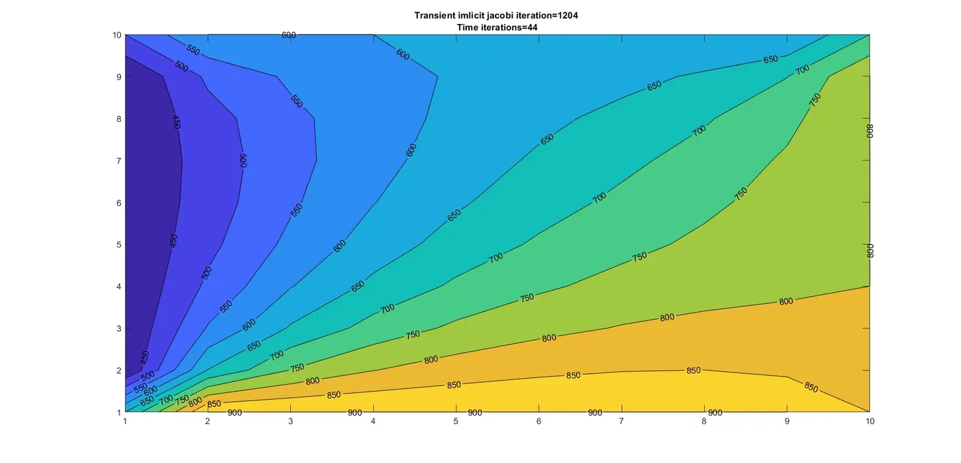
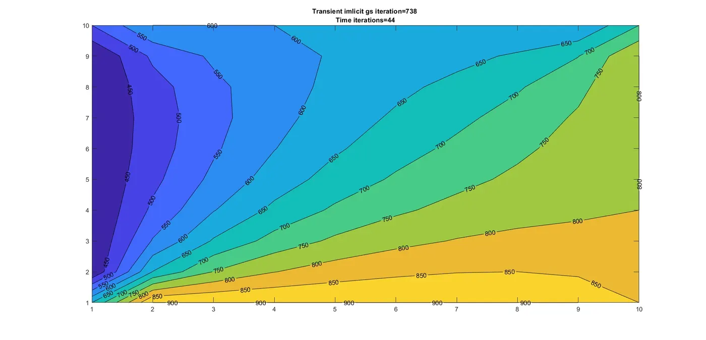
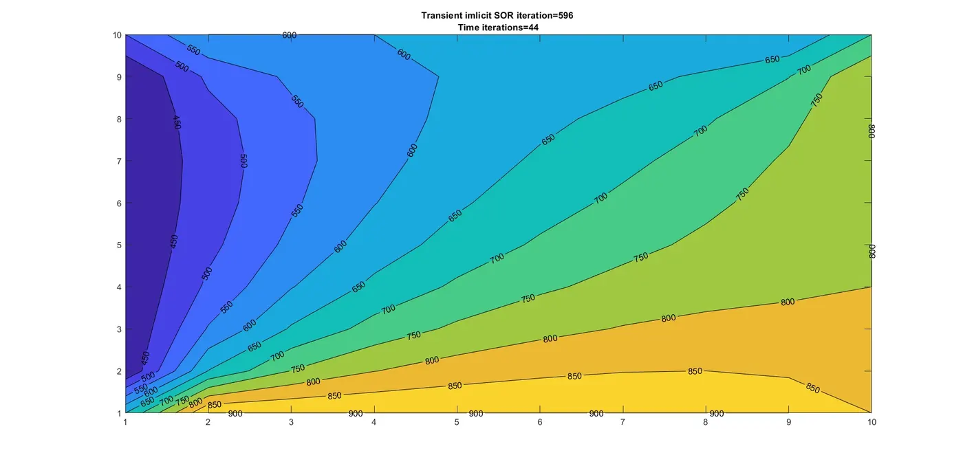
in implicit method the calculation goes step by step approaching through time and gradients well, the end output is same as steady state but the in between flow or the process which the changes go through are clearer in this way.

RESULT :

JACOBI :

GAUSS-SEIDEL :

SOR :

CONCLUSION :

STEADY-STATE HEAT CONDUCTION :

From the above results, the iteration for convergence of plot is very high for the jacobi method when compare with gauss-seidel and sor,by increasing the grid size we can drastically reduce the iteration which as well gives a convergence plot with stability.

TRANSIENT - STATE HEAT CONDUCTION :

The above result shows the convergence of transient heat equation using an explicit and implicit technique.

• unsteady state problems can be solved by both implicit and explicit method.
• for stiff equations required lesser time steps and larger computational time to solve using the explicit method.among implicit solvers,sor gives the result in less time compared to other techniques.it gives stable results irrespective of the CFL number.