Week 5.1 - Mid term project - Solving the steady and unsteady 2D heat conduction problem
Objective :
1. Steady-state analysis & Transient State Analysis
Solve the 2D heat conduction equation by using the point iterative techniques that were taught in the class. The Boundary conditions for the problem are as follows;
Top Boundary = 600 K
Bottom Boundary = 900 K
Left Boundary = 400 K
Right Boundary = 800 K
You will implement the following methods for solving implicit equations.
1. Jacobi
2. Gauss-seidel
3. Successive over-relaxation
Your absolute error criteria are 1e-4.
Steady State Solution
clear all
close all
clc
%initial conditions
%L = 1
nx = 10;
ny = 10;
x = linspace(0,1,nx);
y = linspace(0,1,ny);
dx = x(2) - x(1);
dy = y(2) - y(1);
% given data of boundary condition
% initial temp condition
t = 300*ones(nx,ny);
t(:,1) = 400;
t(1,:) = 600;
t(:,ny) = 800;
t(nx,:) = 900;
% defining the temperature at corner points
t(1,1) = 500;
t(nx,ny) = 850;
t(1,ny) = 700;
t(nx,1) = 650;
dt = 1e-2; %time step
told=t;
error = 100;
tol = 1e-4;
k = 2*(dx^2+dy^2)/(dx^2*dy^2);
% k2 = (dy^2)/(2*(dx^2+dy^2));
method = input('Iterative method = '); %iterative method selection
%JACOBI ITERATIVE METHOD
if (method==1)
tic;
jacobi = 1;
while(error>tol)
for i = 2:(nx-1)
for j = 2:(ny-1)
t(i,j) = (((told(i-1,j)+told(i+1,j))/(dx^2))+((told(i,j+1)+told(i,j-1))/(dy^2)))/k;
end
end
error = max(max(abs(t-told)));
told = t;
jacobi = jacobi+1;
time_taken = toc;
end
%plotting
figure(1)
contourf(x,y,t,'ShowText','on');
colormap(jet);
colorbar;
xlabel('X')
ylabel('Y')
text1 = sprintf('number of iteration = %d', jacobi);
text2 = sprintf('simulation time = %f', time_taken);
title({'Steady state heat condustion profile by jacobi'; text1; text2});
end
%GAUSS-SEIDEL ITERATIVE METHOD
if (method==2)
tic;
gauss = 1;
while(error>tol)
for i = 2:(nx-1)
for j = 2:(ny-1)
t(i,j) = (((t(i-1,j)+told(i+1,j))/(dx^2))+((told(i,j+1)+t(i,j-1))/(dy^2)))/k;
end
end
error = max(max(abs(t-told)));
told = t;
gauss = gauss+1;
time_taken = toc;
end
%plotting
figure(2)
contourf(x,y,t,'ShowText','on');
colormap(jet);
colorbar;
xlabel('X')
ylabel('Y')
text1 = sprintf('number of iteration = %d', gauss);
text2 = sprintf('simulation time = %f', time_taken);
title({'Steady state heat condustion profile by Gauss-Seidel'; text1; text2});
end
%SUCCESSIVE OVER RELAXATION ITERATIVE METHOD
if (method==3)
tic;
sor = 1;
omega = 1.4; %over relaxation factor
while(error>tol)
for i = 2:(nx-1)
for j = 2:(ny-1)
term1 =(t(i-1,j)+told(i+1,j))/(dx^2);
term2 =(told(i,j+1)+t(i,j-1))/(dy^2);
t(i,j) = ((told(i,j)*(1-omega)))+(omega*(term1+term2))/k;
end
end
error = max(max(abs(t-told)));
told = t;
sor = sor+1;
time_taken = toc;
end
%plotting
figure(3)
contourf(x,y,t,'ShowText','on');
colormap(jet);
colorbar;
xlabel('X')
ylabel('Y')
text1 = sprintf('number of iteration = %d', sor);
text2 = sprintf('simulation time = %f', time_taken);
text3 = sprintf('over relaxation factor = %f', omega);
title({'Steady state heat condustion profile by Successive Over Relaxation'; text1; text2; text3});
end
Results
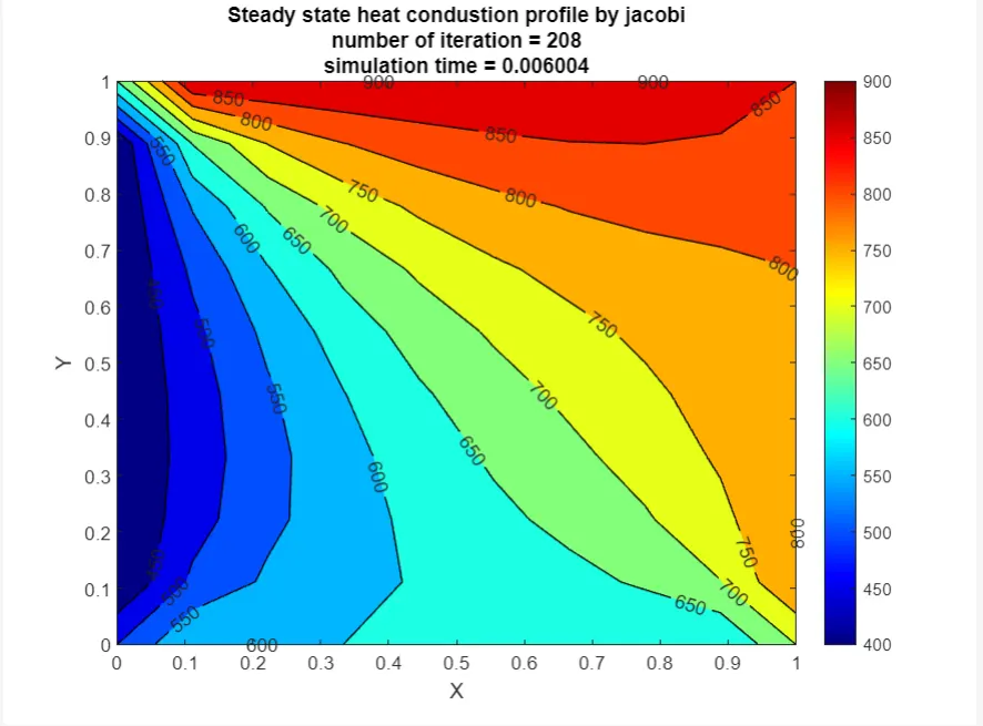
Jacobi
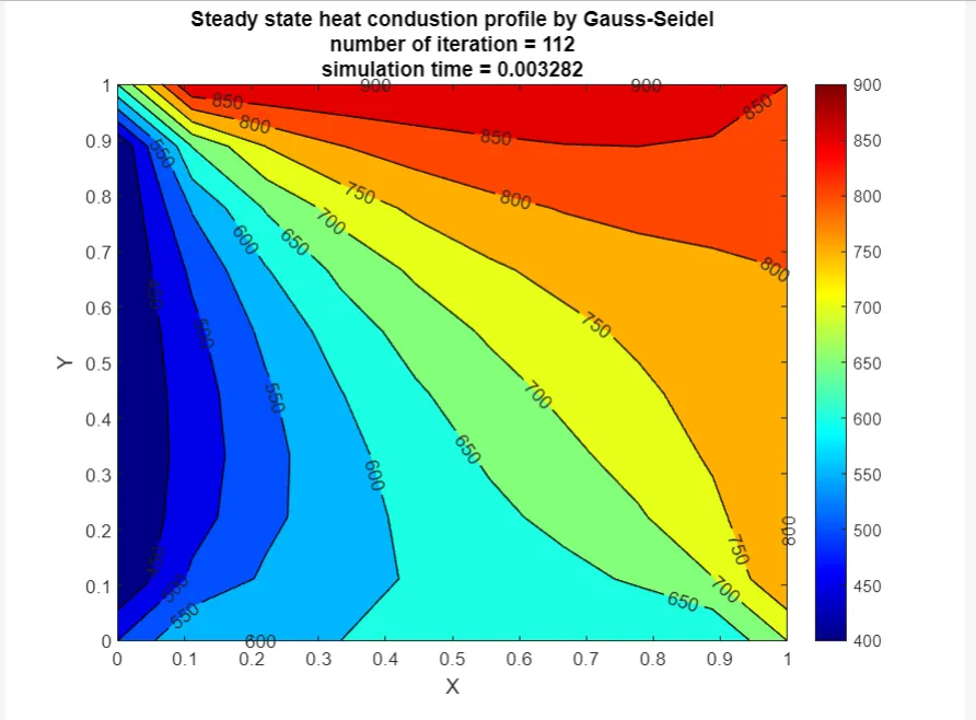
Gauss-Siedel
SOR
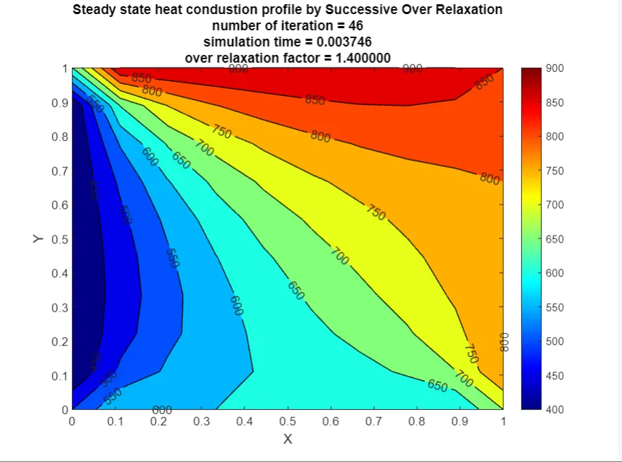
It is evident that SOR computes the desried result in the lowest number of iteration while having time close to gauss sidel mathod.
In Jacobi method the value of the variables is not modified until next iteration, whereas in Gauss-Seidel method the values of the variable are modified as soon as the new value is computed.
Successive Overrelaxation (SOR) can be derived from the Gauss-Seidel method by introducing an extrapolation parameter . For the optimal choice of , SOR may converge faster than Gauss-Seidel by an order of magnitude.
Transient State Solution
Explicit and implicit methods are approaches used in numerical analysis for obtaining numerical approximations to the solutions of time-dependent ordinary and PDEs, as is required in computer simulations of physical process. Explicit methods calculate the state of a system at a later time from the state of the system at the current time, while implicit methods find a solution by solving an equation involving both the current state of the system and the later one
clear all
close all
clc
%initial conditions
%L = 1
nx = 10;
ny = 10;
nt = 300; % No.of steps
x = linspace(0,1,nx);
y = linspace(0,1,ny);
dx = x(2) - x(1);
dy = y(2) - y(1);
% given data of boundary condition
% initial temp condition
t = 300*ones(nx,ny);
t(:,1) = 400;
t(1,:) = 600;
t(:,ny) = 800;
t(nx,:) = 900;
% defining the temperature at corner points
t(1,1) = 500;
t(nx,ny) = 850;
t(1,ny) = 700;
t(nx,1) = 650;
dt = 0.01; %time step
told=t;
alpha = 0.3; % Thermal diffusivity
tprev_dt = told;
tol = 1e-4;
k1 = alpha*dt/(dx^2);
k2 = alpha*dt/(dy^2);
method = input('Iterative method = '); %iterative method selection
%JACOBI ITERATIVE METHOD
if (method==1)
tic;
jacobi = 1;
for p = 1:nt
error =100;
while(error>tol)
for i = 2:(nx-1)
for j = 2:(ny-1)
term1 = (1+(2*k1)+(2*k2))^-1;
term2 = k1*term1;
term3 = k2*term1;
h = (told(i-1,j)+told(i+1,j));
v = (told(i,j+1)+told(i,j-1));
t(i,j) = ((tprev_dt(i,j)*term1)+(h*term2)+(v*term3));
end
end
error = max(max(abs(t-told)));
told = t;
jacobi = jacobi+1;
end
tprev_dt = t ;
end
time_taken = toc;
%plotting
figure(1)
contourf(x,y,t,'ShowText','on');
colormap(jet);
colorbar;
xlabel('X')
ylabel('Y')
text1 = sprintf('number of iteration = %d', jacobi);
text2 = sprintf('simulation time = %f', time_taken);
title({'Transient state heat conduction profile Implicit-Jacobi'; text1; text2});
end
%GAUSS-SEIDEL ITERATIVE METHOD
if (method==2)
tic;
gauss = 1;
for p = 1:nt
error =100;
while(error>tol)
for i = 2:(nx-1)
for j = 2:(ny-1)
term1 = (1+(2*k1)+(2*k2))^-1;
term2 = k1*term1;
term3 = k2*term1;
h = (t(i-1,j)+told(i+1,j));
v = (told(i,j+1)+t(i,j-1));
t(i,j) = ((tprev_dt(i,j)*term1)+(h*term2)+(v*term3));
end
end
error = max(max(abs(t-told)));
told = t;
gauss = gauss+1;
end
tprev_dt = t;
end
time_taken = toc;
%plotting
figure(1)
contourf(x,y,t,'ShowText','on');
colormap(jet);
colorbar;
xlabel('X')
ylabel('Y')
text1 = sprintf('number of iteration = %d', gauss);
text2 = sprintf('simulation time = %f', time_taken);
title({'Transient state heat conduction profile Implicit-Gauss-seidel'; text1; text2});
end
%SUCCESSIVE OVER RELAXATION ITERATIVE METHOD
if (method==3)
tic;
sor = 1;
omega = 1.2; % Over relaxation factor
for p = 1:nt
error =100;
while(error>tol)
for i = 2:(nx-1)
for j = 2:(ny-1)
term1 = (1+(2*k1)+(2*k2))^-1;
term2 = k1*term1;
term3 = k2*term1;
h = (t(i-1,j)+told(i+1,j));
v = (told(i,j+1)+t(i,j-1));
t(i,j) = (told(i,j)*(1-omega))+(omega*((tprev_dt(i,j)*term1)+(h*term2)+(v*term3)));
end
end
error = max(max(abs(t-told)));
told = t;
sor = sor+1;
end
tprev_dt = t ;
end
time_taken = toc;
%plotting
figure(1)
contourf(x,y,t,'ShowText','on');
colormap(jet);
colorbar;
xlabel('X')
ylabel('Y')
text1 = sprintf('number of iteration = %d', sor);
text2 = sprintf('simulation time = %f', time_taken);
title({'Transient state heat conduction profile Implicit-SOR'; text1; text2});
end
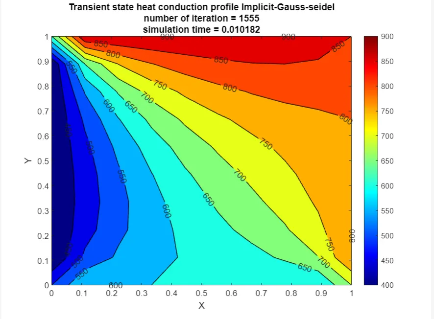
Results
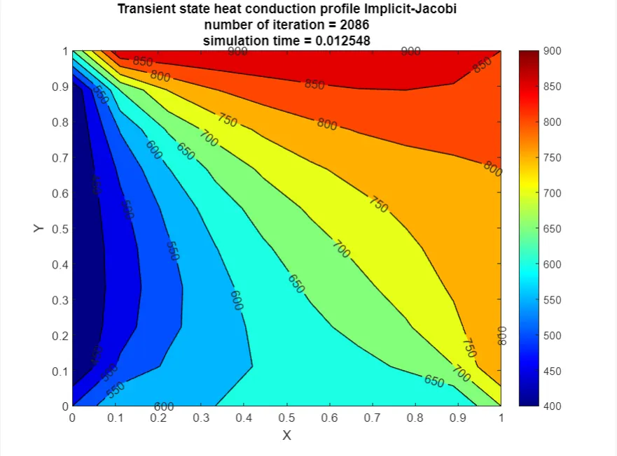
Implicit Jacobi
Implicit Gauss-Siedel
Implicit SOR
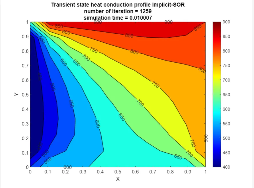
Successive Over Relaxation method provides the desired result much faster and with less computations than the other two methods.