Challenge

Week 5.1 - Mid term project - Solving the steady and unsteady 2D heat conduction problem

SSuhail Ahmed S6 Oct 2023

Solving steady and unsteady 2D heat conduction problem

Aim: To solve the 2D heat conduction problem for both steady and unsteady condition by using the point iterative method. Compare the plots of steady and unsteady condition.

Objective:

Stimulate steady state analysis and transient state analysis.
The boundary conditions top = 600k, bottom = 900k, left = 400k and right = 800k.
To implement the following methods for solving implicit equations. They are Jacobi, gauss-seidel and successive over-relaxation.
Absolute error criteria is 1e-4.
To write code for both implicit and explicit schemes.
Compare the convergence rate [Number of iterations] of the steady state and transient [implicit and explicit] simulations and justify the numerics.

Introduction:

In this challenge we are going see major two types of analysis steady and unsteady(transient) condition.

Steady condition: A steady state is one in which the conditions (velocity, pressure and cross-section) may vary from point to point but doesn't change with time.

Unsteady or Transient condition: A unsteady state is one in which the conditions (velocity, pressure and cross-section) vary from point to point and change with respect to time.

In numerical analysis for obtaining numerical approximations to the solutions of the time-dependent ordinary and partial differential equation mainly two approaches are used. They are Explicit and Implicit approach.

Explicit Approach: We solve later time-step values (n+1) with current time-step values (n). The explicit approach is a direct approach which doesn't need any iterative solver for convergence loop.

Implicit approach: We solve later time-step values (n+1) with both current time-step values (n) and later time-step values (n+1). The implicit is an indirect method which needs iterative solver for convergence loop.

Iterative solver: It refers to wide range of technique that use successive approximations to obtain more accurate solution to linear system at each time-steps. Some of the iterative methods are,

Jacobi method
Gauss-Seidel method
Successive Over-Relaxation method

Solutions:

Here we are going to solve the 2D heat conduction problem for both steady and unsteady condition by using the point iterative method. stimulate steady state analysis and transient state analysis. For implicit method use following iterative methods jacobi, gauss-seidel and successive over-relaxation.

Steady State Analysis:

2D heat conduction equation, ∇²T = 0.

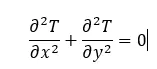
Then expand above equation terms using central differencing scheme,

Rearrange the equation,

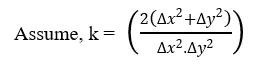
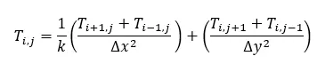
Above equation written in Jacobi form,

Gauss-seidel form,

Successive over-relaxation form,

Code for Steady State Analysis:

clear all

close all

clc

% input values for steady state conduction

nx = 10;

ny = 10;

x = linspace(0,1,nx);

y = linspace(0,1,ny);

% grid points spacing

dx = x(2) - x(1);

dy = y(2) - y(1);

% boundary condition;

T = 300*ones(nx,ny);

T(:,1) = 400;

T(1,:) = 600;

T(:,ny) = 800;

T(nx,:) = 900;

% computing the cornering temperature

T(1,1) = 500;

T(nx,ny) = 850;

T(1,ny) = 700;

T(nx,1) = 650;

% timestep and initial temperature condition

dt = 1e-2;

Told=T;

% sample error,tolerance_value and over relaxation factor

error = 9e9;

tolerance_value = 1e-4;

omega = 1.2;

% for calculating k value

k = 2*((dx^2)+(dy^2))/((dx^2)*(dy^2));

% selecting the iterative solver

iterative_solver = input('Iterative method =');

% Jacobi Method

if iterative_solver==1

jacobi_iter = 1;

while(error>tolerance_value)

for i = 2:(nx-1)

for j = 2:(ny-1)

term1=(Told(i+1,j)+Told(i-1,j))/(k*dx^2);

term2=(Told(i,j+1)+Told(i,j-1))/(k*dy^2);

T(i,j)=(term1+term2);

end

error = max(max(abs(Told-T)));

Told = T;

jacobi_iter = jacobi_iter+1;

end

% Plotting the contour

figure(1)

contourf(x,y,flip(T),'ShowText','on');

colormap(jet);

colorbar;

xlabel('X')

ylabel('Y')

text1 = sprintf('number of iteration = %d', jacobi_iter);

title({'Steady state heat conduction by Jacobi'; text1;});

end

% Gauss-Seidel Method

if iterative_solver==2

gs_iter = 1;

while(error>tolerance_value)

for i = 2:(nx-1)

for j = 2:(ny-1)

term1=(Told(i+1,j)+T(i-1,j))/(k*dx^2);

term2=(Told(i,j+1)+T(i,j-1))/(k*dy^2);

T(i,j)=(term1+term2);

end

error = max(max(abs(Told-T)));

Told = T;

gs_iter = gs_iter+1;

end

% Plotting the contour

figure(2)

contourf(x,y,flip(T),'ShowText','on');

colormap(jet);

colorbar;

xlabel('X')

ylabel('Y')

text1 = sprintf('number of iteration = %d', gs_iter);

title({'Steady state heat conduction by Gauss-Seidel'; text1});

end

% Successive Over Relaxation Method

if iterative_solver==3

SOR_iter = 1;

while(error>tolerance_value)

for i = 2:(nx-1)

for j = 2:(ny-1)

term1=(Told(i+1,j)+T(i-1,j))/(k*dx^2);

term2=(Told(i,j+1)+T(i,j-1))/(k*dy^2);

T(i,j)=(Told(i,j)*(1-omega))+(omega*(term1+term2));

end

error = max(max(abs(Told-T)));

Told = T;

SOR_iter = SOR_iter+1;

end

% Plotting the contour

figure(3)

contourf(x,y,flip(T),'ShowText','on');

colormap(jet);

colorbar;

xlabel('X')

ylabel('Y')

text1 = sprintf('number of iteration = %d', SOR_iter);

title({'Steady state heat conduction profile by SOR'; text1;});

end

Results:

Jacobi output:

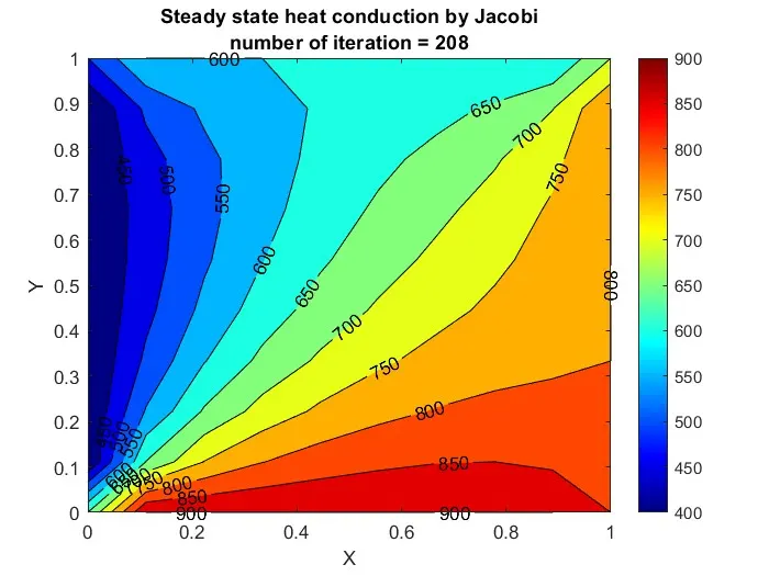
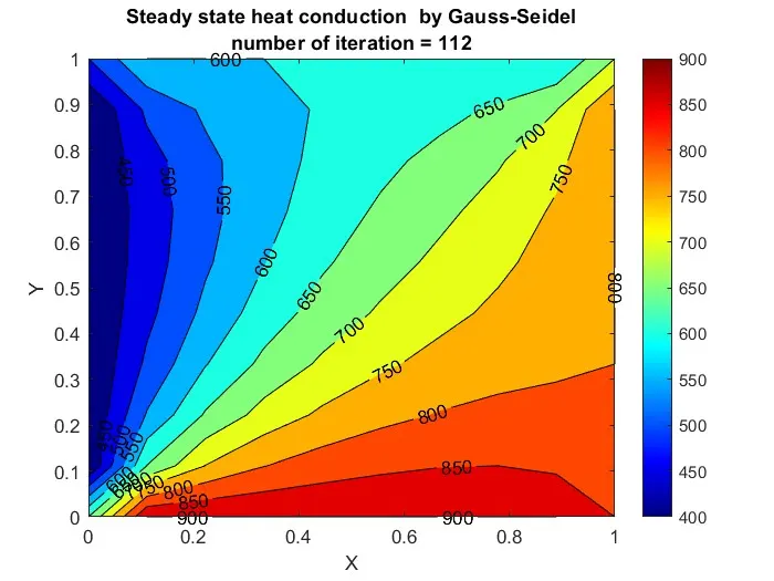
Gauss-seidel output:

Successive over-relaxation output:

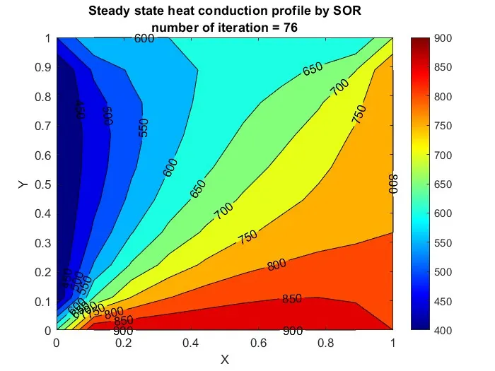
From the above results, we conclude that the solution converges more faster in successive over-relaxation method compared to Jacobi and gauss-seidel iterative methods.

Transient State Analysis (Implicit):

2D heat conduction equation,

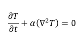
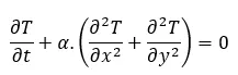
Then expand above equation terms using central differencing scheme,

Rearrange the equation,

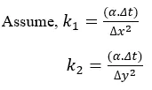
move n+1 terms to L.H.S,

take T(i,j) term common out,

Above equation written in Jacobi form,

Gauss-seidel form,

Successive over-relaxation form,

Code for Transient State Analysis (Implicit):

clear all

close all

clc

% input values for transient heat conduction

nx = 10;

ny = 10;

nt = 300;

x = linspace(0,1,nx);

y = linspace(0,1,ny);

% grid points spacing

dx = x(2) - x(1);

dy = y(2) - y(1);

% boundary condition;

T = 300*ones(nx,ny);

T(:,1) = 400;

T(1,:) = 600;

T(:,ny) = 800;

T(nx,:) = 900;

% computing the cornering temperature

T(1,1) = 500;

T(nx,ny) = 850;

T(1,ny) = 700;

T(nx,1) = 650;

% timestep and initial temperature condition

dt = 1e-2;

Told=T;

T_prev=Told;

% sample error,tolerance_value and over relaxation factor

error = 9e9;

tolerance_value = 1e-4;

alpha = 0.3;

omega = 1.2;

% for calculating k1 and k2 value

k1 = alpha*dt/(dx^2);

k2 = alpha*dt/(dy^2);

% selecting the iterative solver

iterative_solver = input('Iterative method =');

% Jacobi Method

if iterative_solver==1

tic

jacobi_iter = 1;

for p = 1:nt

error =9e9;

while(error>tolerance_value)

for i = 2:(nx-1)

for j = 2:(ny-1)

term1 = (1+(2*k1)+(2*k2))^-1;

term2 = k1*term1;

term3 = k2*term1;

H = (Told(i-1,j)+Told(i+1,j));

V = (Told(i,j+1)+Told(i,j-1));

T(i,j) = ((T_prev(i,j)*term1)+(H*term2)+(V*term3));

end

error = max(max(abs(Told-T)));

Told = T;

jacobi_iter = jacobi_iter+1;

end

T_prev = T;

end

simulation_time = toc;

% Plotting the contour

figure(1)

contourf(x,y,flip(T),'ShowText','on');

colormap(jet);

colorbar;

xlabel('X')

ylabel('Y')

text1 = sprintf('number of iteration = %d', jacobi_iter);

text2 = sprintf('Simulation time = %f',simulation_time);

title({'Transient state heat conduction by Jacobi (implicit)'; text1;text2;});

end

% Gauss-Seidel Method

if iterative_solver==2

tic

gs_iter = 1;

for p = 1:nt

error =9e9;

while(error>tolerance_value)

for i = 2:(nx-1)

for j = 2:(ny-1)

term1 = (1+(2*k1)+(2*k2))^-1;

term2 = k1*term1;

term3 = k2*term1;

H = (T(i-1,j)+Told(i+1,j));

V = (Told(i,j+1)+T(i,j-1));

T(i,j) = ((T_prev(i,j)*term1)+(H*term2)+(V*term3));

end

error = max(max(abs(Told-T)));

Told = T;

gs_iter = gs_iter+1;

end

T_prev = T;

end

simulation_time = toc;

% Plotting the contour

figure(2)

contourf(x,y,flip(T),'ShowText','on');

colormap(jet);

colorbar;

xlabel('X')

ylabel('Y')

text1 = sprintf('number of iteration = %d', gs_iter);

text2 = sprintf('Simulation time = %f',simulation_time);

title({'Transient state heat conduction by Gauss-Seidel (implicit)'; text1;text2;});

end

% Successive Over Relaxation Method

if iterative_solver==3

tic

SOR_iter = 1;

for p = 1:nt

error =9e9;

while(error>tolerance_value)

for i = 2:(nx-1)

for j = 2:(ny-1)

term1 = (1+(2*k1)+(2*k2))^-1;

term2 = k1*term1;

term3 = k2*term1;

H = (T(i-1,j)+Told(i+1,j));

V = (Told(i,j+1)+T(i,j-1));

T(i,j) = (Told(i,j)*(1-omega))+(omega*((T_prev(i,j)*term1)+(H*term2)+(V*term3)));

end

error = max(max(abs(Told-T)));

Told = T;

SOR_iter = SOR_iter+1;

end

T_prev = T;

end

simulation_time = toc;

% Plotting the contour

figure(3)

contourf(x,y,flip(T),'ShowText','on');

colormap(jet);

colorbar;

xlabel('X')

ylabel('Y')

text1 = sprintf('number of iteration = %d', SOR_iter);

text2 = sprintf('Simulation time = %f',simulation_time);

title({'Transient state heat conduction profile by SOR (implicit)'; text1;text2;});

end

Results:

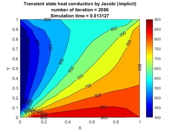
Jacobi output:

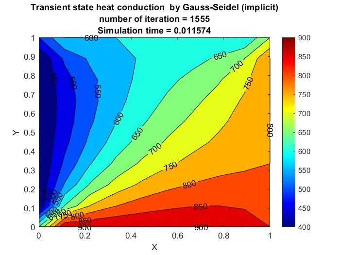
Gauss-seidel output:

Successive over-relaxation output:

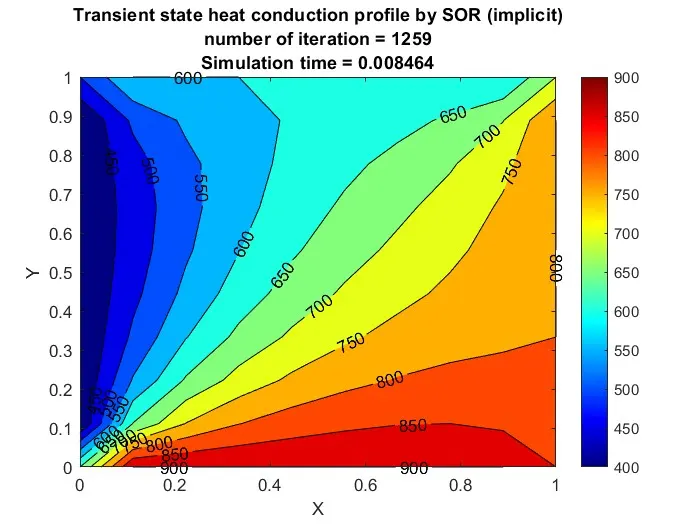
From the above results, we conclude that the solution converges more faster in successive over-relaxation method compared to Jacobi and gauss-seidel iterative methods. The successive over-relaxation method takes less run time for simulation.

Transient State Analysis (Explicit):

2D heat conduction equation,

Then expand above equation terms using central differencing scheme,

Rearrange the equation,

take T(i,j) term common out,

Above equation is the transient explicit 2D heat conduction equation.

Code for Transient State Analysis (Explicit):

clear all

close all

clc

% input values for transient heat conduction

nx = 10;

ny = 10;

nt = 300;

x = linspace(0,1,nx);

y = linspace(0,1,ny);

% grid points spacing

dx = x(2) - x(1);

dy = y(2) - y(1);

% boundary condition;

T = 300*ones(nx,ny);

T(:,1) = 400;

T(1,:) = 600;

T(:,ny) = 800;

T(nx,:) = 900;

% computing the cornering temperature

T(1,1) = 500;

T(nx,ny) = 850;

T(1,ny) = 700;

T(nx,1) = 650;

% timestep and initial temperature condition

dt = 1e-2;

Told=T;

% alpha value

alpha = 0.3;

% for calculating k1 and k2 value

k1 = alpha*dt/(dx^2);

k2 = alpha*dt/(dy^2);

% Explicit method

tic

Explicit_iter = 1;

for p = 1:nt

for i = 2:(nx-1)

for j = 2:(ny-1)

H = (Told(i-1,j)+Told(i+1,j));

V = (Told(i,j+1)+Told(i,j-1));

term1 = k1*H;

term2 = k2*V;

T(i,j) = (Told(i,j)*(1-2*k1-2*k2)+term1+term2);

end

error = max(max(abs(Told-T)));

Told = T;

Explicit_iter=Explicit_iter+1;

end

simulation_time = toc;

% Plotting the contour

figure(1)

contourf(x,y,flip(T),'ShowText','on');

colormap(jet);

colorbar;

xlabel('X')

ylabel('Y')

text1 = sprintf('number of iteration = %d', Explicit_iter);

text2 = sprintf('Simulation time = %f',simulation_time);

title({'Transient state heat conduction by Explicit)'; text1;text2;});

Result:

Explicit output:

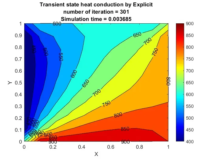
From the above results, we conclude that the solution converges more faster in explicit compared to implicit method. The explicit method take less run time for simulation.

Conclusion:

For steady state analysis, successive over-relaxation method converges more faster and take less run time for stimulation.
For Transient state analysis, explicit method converges more faster and take less run time for stimulation.
Explicit method provides more accurate solution with less run time compared to implicit method.

Week 5.1 - Mid term project - Solving the steady and unsteady 2D heat conduction problem

Solving steady and unsteady 2D heat conduction problem

Ship work like this
in your own course.

Talk to a career counsellor

Solving steady and unsteady 2D heat conduction problem

Ship work like thisin your own course.

Talk to a career counsellor

Ship work like this
in your own course.