Week 5.1 - Mid term project - Solving the steady and unsteady 2D heat conduction problem

Objective: Steady state analysis & Transient State Analysis of 2D heat conduction equation.

The Boundary conditions for the problem are as follows;

Top Boundary = 600 K

Bottom Boundary = 900 K

Left Boundary = 400 K

Right Boundary = 800 K

Theory:

Steady heat conduction equation is:

`(del^2T)/(delx^2)+(del^2T)/(dely^2)=0`

After discritisation the equation become.

`((T(i+1,j)-2*T(i,j)+T(i-1,j))/(Deltax^2))+((T(i,j+1)-2*T(i,j)+T(i,j-1))/(Deltay^2))=0`

.After solving the equaation and separating the T(i,j)

`k=(2*(Deltax^2+Deltay^2))/(Deltax^2*Deltay)^2`

`(((T(i+1,j)+T(i-1,j))/(Deltax^2))+((T(i,j+1)-+T(i,j-1))/(Deltay^2)))*(1/k)=T(i,j)`

Jocobi method:

• Jocobi method is a ittrative method in which we gausse a value for all the nodes we have to find the value.
• Then calculate the value of all node by useing the gausse value.
• In the Jocobi method we solve the present itrration by useing previose ittration value.
• The calculate the racidual by subtracting the gausse value and present value.
• then check residual is within the tolerance level or not.
• if the residual was not within the limit,do the ittration again.
• then check the resdual by compering the previous itrration value and present ittration value.
• ittrate till residual should within the tolerance limit.

`(((Told(i+1,j)+Told(i-1,j))/(Deltax^2))+((Told(i,j+1)+Told(i,j-1))/(Deltay^2)))*(1/k)=T(i,j)`

Gauss-seidel:

• Gauss-seidal method is a ittrative method in which we gausse a value for all the nodes we have to find the value.
• Then calculate the value of all node by useing the gausse value.
• In the Gauss-seidal method we solve the present itrration by useing present ittration value.
• The calculate the racidual by subtracting the gausse value and present value.
• then check residual is within the tolerance level or not.
• if the residual was not within the limit,do the ittration again.
• then check the resdual by compering the previous itrration value and present ittration value.
• ittrate till residual should within the tolerance limit.

`(((T(i+1,j)+T(i-1,j))/(Deltax^2))+((T(i,j+1)-+T(i,j-1))/(Deltay^2)))*(1/k)=T(i,j)`

sucssive over relaxation:

• The Gauss–Seidel method described previously generally does not converge sufficiently fast. SOR is a method that can accelerate the convergence. 

The liner from of equation is:

`(((T(i+1,j)+T(i-1,j))/(Deltax^2))+((T(i,j+1)-+T(i,j-1))/(Deltay^2)))*(1/k)=T(i,j)`

After Addiing and subtracting the T(i,J) we get

`T(i,j)+(((T(i+1,j)+T(i-1,j))/(Deltax^2))+((T(i,j+1)-+T(i,j-1))/(Deltay^2))+k*T(i,j))*(1/k)=T(i,j)`

This is gauss-Seidel equation to increses the convergence we multiply ω(relaxation parameter).

`T(i,j)+(((T(i+1,j)+T(i-1,j))/(Deltax^2))+((T(i,j+1)+T(i,j-1))/(Deltay^2))-k*T(i,j))*(omega/k)=T(i,j)`

• The range 0 < ω < 1 xss=removed>

Transient State heat conduction equation:

`(del^2T)/(delx^2)+(del^2T)/(dely^2)=1/alpha*((delT)/(delt))`

We can discretize in two way one is implicity method and explicity method.

implicity method

 In this method we use the present timestep value to discritize differencial equation.

Then disctise the above equation:

^{`((T1(i+1,j)-2*T1(i,j)+T1(i-1,j))/(Deltax^2))+((T1(i,j+1)-2*T1(i,j)+T1(i,j-1))/(Deltay^2))=1/alpha*(T1(i,j)-T(i,j))/(Deltat)`}

^{Here T1 is the present time step in which we have to calculate T1(i,j),T is previous time step value of that node.}

^{after some simplification we found:}

^{`k1=(alpha*Deltat)/(Deltax^2)`}

^{`k2=(alpha*Deltat)/(Deltay^2)`}

^{`T1(i,j)=(1/(1+(2*k1)+(2*k2)))*(T(i,j)+k1*(T1(i-1,j)+T1(i+1,j))+k2*(T1(i,j+1)+T1(i,j-1)))`}

• If we use jocobi method for ittrative solver then we take previous ittration value.

^{`T1(i,j)=(1/(1+(2*k1)+(2*k2)))*(T(i,j)+k1*(Told1(i-1,j)+Told1(i+1,j))+k2*(Told1(i,j+1)+Told1(i,j-1)))`}

• Told1 is previous ittration value for present time step.
• For Gauss_seidel method we use prasent ittration value.
• For SOR method we apply the ω(relaxation parameter) then the equation become:

`T1(i,j)=(1-omega)*Told1(i,j)+(omega/(1+(2*k1)+(2*k2)))*(T(i,j)+k1*(Told1(i-1,j)+Told1(i+1,j))+k2*(Told1(i,j+1)+Told1(i,j-1)))`

^{Explicity Method:}

 In this method we use the previous timestep value to discritize differencial equation.

Then disctise the above equation:

^{`((T(i+1,j)-2*T(i,j)+T(i-1,j))/(Deltax^2))+((T(i,j+1)-2*T(i,j)+T(i,j-1))/(Deltay^2))=alpha*(T1(i,j)-T(i,j))/(Deltat)`}

after some simplification we found:

`k1=(alpha*Deltat)/(Deltax^2)`

`k2=(alpha*Deltat)/(Deltay^2)`

`T1(i,j)=((1-(2*k1)-(2*k2))*T(i,j)+k1*(T(i-1,j)+T(i+1,j))+k2*(T(i,j+1)+T(i,j-1)))`

• T1 is prasent timestep and T is the previous time step.
• Here ittrative method is not effective because here we calculate the  present value by useing the past time stap value so there is no change of past time stap value after every ittration.

Matlab code for Steady state Heat conduction equation:

clear all

close all

clc

alpha=1.2;

% Domain and dicretization length

nx=10;

ny=10;

domain_length = 1;

%value of x and y at nodes in a discretization plane

x = linspace(0,domain_length,nx);

y = linspace(0,domain_length,ny);

dx = domain_length/(nx-1);

dy = domain_length/(ny-1);

t=ones(nx,ny);

t(1,:)=600;

t(end,:)=900;

t(:,1)=400;

t(:,end)=800;

told=t

%constant

K = (2*(dx^2+dy^2))/(dx^2*dy^2);

t_pre=t

error=1

tol=1e-4

no_ittration=1;

method=input('if jocobo 1, guss elmination 2,sor 3')

%jocobi method

if method==1

while(error>tol)

        for i = 2:nx-1

            for j = 2:ny-1

            term1 = (told(i+1,j)+told(i-1,j))/dx^2;

            term2 = (told(i,j+1)+told(i,j-1))/dy^2;

            t(i,j) = (term1+term2)/K;

            end

        end

        error = max(max(abs(told-t)));

        

        % to upadte the previous velcity with new velocity

        %got from the iteration

        told = t;

        no_ittration = no_ittration+1

end

end

%Gauss_seidal method

if method==2

while(error>tol)

        for i = 2:nx-1

            for j = 2:ny-1

            term1 = (t(i+1,j)+t(i-1,j))/dx^2;

            term2 = (t(i,j+1)+t(i,j-1))/dy^2;

            t(i,j) = (term1+term2)/K;

            end

        end

        error = max(max(abs(told-t)));

        

        % to upadte the previous velcity with new velocity

        %got from the iteration

        told = t;

        no_ittration = no_ittration+1

end

end

% Sucssive over relaxation

if method==3

    omega=1.5

while(error>tol)

        for i = 2:nx-1

            for j = 2:ny-1

            term1 = (t(i+1,j)+t(i-1,j))/dx^2;

            term2 = (t(i,j+1)+t(i,j-1))/dy^2;

            t(i,j) = ((omega*(term1+term2))/K)+((1-omega)*told(i,j));

            end

        end

        error = max(max(abs(told-t)));

        

        % to upadte the previous velcity with new velocity

        %got from the iteration

        told = t;

        no_ittration = no_ittration+1

end

end

[X,Y] = meshgrid(x,y);

contourf(X,Y,t)

colorbar

set(gca,'ydir','reverse')

Output:

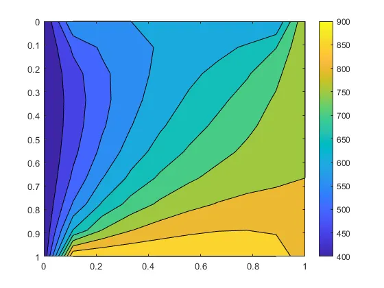
For jocobi method no of ittration was:217

For gauss_seidal method no of ittration was:117

For SOR method(with ω=1.5) no of ittration was:30

For SOR method(with ω=1.25) no of ittration was:70

For SOR method(with ω=1.75) no of ittration was:62

Output analysis :

• In the tempreture profile show that tempreture distribution buttom of the plate to the left of the plate, because buttom of the plate have higher temprature(900K) and left side has lowest tempreture(400).
• The output for all the method are same.
• Here jocobi method need more no of ittretion as compare to the other method,because it use always use old values.
• In SOB method the value converge with less ittration but it also depeand on the ω value

Matlab code for Transent heat conduction equation useing implicity discritisation: 

 close all

clear all

clc

%solve second order 1d pd

%solve d^2u/dx^2

%input

alpha=0.1;

% Domain and dicretization length

nx=10;

ny=10;

domain_length = 1;

%value of x and y at nodes in a discretization plane

x = linspace(0,domain_length,nx);

y = linspace(0,domain_length,ny);

dx = domain_length/(nx-1);

dy = domain_length/(ny-1);

t=ones(nx,ny);

t(1,:)=600;

t(end,:)=900;

t(:,1)=400;

t(:,end)=800;

told=t;

t_pre=t;

no_of_time_step=12

dt=0.1;

no_of_ittration=0

k1=(alpha*dt)/(dx^2);

k2=(alpha*dt)/(dy^2);

term1=(1+(2*k1)+(2*k2))^-1;

term2=k1*term1;

term3=k2*term1;

%input the method

method=input('if jocobo 1, guss elmination 2,sob 3')

if(method==1)

%for the time loop

for n=2:no_of_time_step

%to ittrate till tolerance

 error=1

tol=1e-4

while(error>tol)

   for i=2:nx-1

       for j=2:ny-1

           H=told(i-1,j)+told(i+1,j);

           v=told(i,j-1)+told(i,j+1);

           t(i,j)=(t_pre(i,j)*term1)+(H*term2)+(v*term3);

       end

   end   

error=max(max(abs(told-t)))

no_of_ittration=no_of_ittration+1

told=t;

end

t_pre=t;

end

end

%For gauss_sedial method

if(method==2)

%for the time loop

for n=2:no_of_time_step

    error=1

tol=1e-4

%to ittrate till tolerance

while(error>tol)

   for i=2:nx-1

       for j=2:ny-1

           H=t(i-1,j)+t(i+1,j);

           v=t(i,j-1)+t(i,j+1);

           t(i,j)=(t_pre(i,j)*term1)+(H*term2)+(v*term3);

       end

   end

   error=max(max(abs(told-t)))

no_of_ittration=no_of_ittration+1

told=t;

end

t_pre=t;

end

end

%SOB method

if(method==3)

    omega=1.5

%for the time loop

for n=2:no_of_time_step

    error=1

tol=1e-4

%to ittrate till tolerance

while(error>tol)

   for i=2:nx-1

       for j=2:ny-1

           H=t(i-1,j)+told(i+1,j);

           v=t(i,j-1)+told(i,j+1);

           t(i,j)=(omega*((t_pre(i,j)*term1)+(H*term2)+(v*term3)))+((1-omega)*told(i,j));

       end

   end

   error=max(max(abs(told-t)))

no_of_ittration=no_of_ittration+1

told=t;

end

t_pre=t;

end

end

[X,Y] = meshgrid(x,y);

contourf(X,Y,t)

colorbar

set(gca,'ydir','reverse')

Output:

at no of time step:12

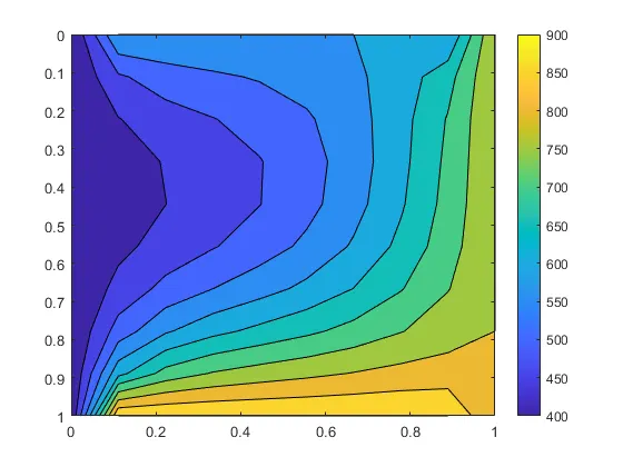
For jocobi method no of ittration is:421

For gauss_seidal method no of ittration was:250

For SOR method(with ω=1.5) no of ittration was:272

For SOR method(with ω=1.2) no of ittration was:168

at no of time step:25

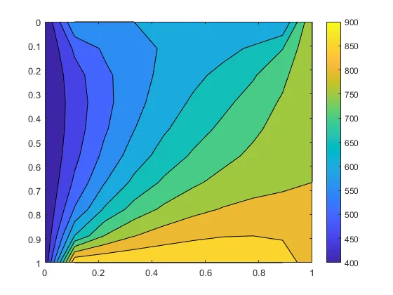
For jocobi method no of ittration is:835

For gauss_seidal method no of ittration was:499

For SOR method(with ω=1.5) no of ittration was:570

For SOR method(with ω=1.2) no of ittration was:330

Output analyis:

• The tempreture distribution will change with time,There is no change of tempreture distribution after 25 no of time step.
• Jocobi method need higher no of ittration.
• The no of ittration in the SOB method is depeand upon the ω.so at ω=1.5 need more no itrration then gauss_seidal method.

Matlab code for Explicit method:

close all

clear all

clc

%solve second order 1d pd

%solve d^2u/dx^2

%input

alpha=0.1;

% Domain and dicretization length

nx=10;

ny=10;

domain_length = 1;

%value of x and y at nodes in a discretization plane

x = linspace(0,domain_length,nx);

y = linspace(0,domain_length,ny);

dx = domain_length/(nx-1);

dy = domain_length/(ny-1);

t=ones(nx,ny);

t(1,:)=600;

t(end,:)=900;

t(:,1)=400;

t(:,end)=800;

told=t;

t_pre=t;

no_of_time_step=25

dt=0.1;

no_of_ittration=0

k1=(alpha*dt)/(dx^2);

k2=(alpha*dt)/(dy^2);

term1=1-(2*k1)-(2*k2);

%for the time loop

for n=2:no_of_time_step

%to ittrate till tolerance

   for i=2:nx-1

       for j=2:ny-1

           H=(t_pre(i-1,j)+t_pre(i+1,j))*k1;

           v=(t_pre(i,j-1)+t_pre(i,j+1))*k2;

           t(i,j)=(t_pre(i,j)*term1)+H+v;

       end

   end   

error=max(max(abs(told-t)))

no_of_ittration=no_of_ittration+1

t_pre=t;

end

[X,Y] = meshgrid(x,y);

contourf(X,Y,t)

colorbar

set(gca,'ydir','reverse')

Output:

At time step size:0.1 and number of timestep:25

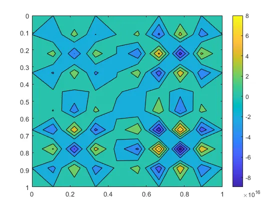
At time step size:0.01and number of timestep:25

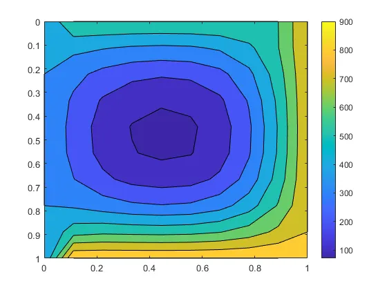
At time step size:0.01and number of timestep:200

• At the time stap size 0.1 the K1+k2>1 so the the solution was unstable.
• Because of the solver is explicit there is no effect on the t value after every ittration(here we use prebious time stap value).So ittration loop is not there.
• At time step size 0.01 and no of time step 200.