Week 5.1 - Mid term project - Solving the steady and unsteady 2D heat conduction problem

Solving the steady and unsteady 2D heat conduction Equation

For an unsteady state the 2-D heat conduction equation is represented as :

∂T/∂t = α . (∂^2 T/∂x^2 + ∂^2 T/∂y^2)

For a steady state condition equation is represnted as:

(∂^2 T/∂x^2 + ∂^2 T/∂y^2) = 0

These equation are partial differential eqaution and hence the numerical discretization techniques can be used to solve these equation useing the numerical analysis.

Jacobi Method :

Jacobi iterative method is consider as an iterative algorithem which is used for determining the solution for the system of linear equation. In this method an approximate value is used and then the entire equation is solved using this guess value , Until it converges the process is iterated. With the jacobi method the values of T^n obtained in the n th iteration remains unchanged until the entre (n+ 1) th iteration has been calculated.

Gauss seidel method :

The gauss seidal method we use the new values T^n+1 as soon as they are known. For example , once we have computed T^n+1 from the first equation its value id the second equation to obtain the new T2 ^n+1 and so on.

In similar words the difference between the gauss seidal and jaccobi method is that the  jacobi method uses the obtained from the previous step while the gauss seidal method always applies the latest utated values during the iterative procedures.

Successive over relaxtion method (SOR)

This iterative method uses a value ω to guess seidel metho formula i this manner the gauss seidal method formula the values are computed.

T^n+1 = T^n . (1-ω) + ω .(T  GS)

In this T GS is the value computed using the gauss sedel iteration method formula . in this manner the gauss seidel method is extended to the relaxation method.

Transient Analysis using the explicit scheme :

Since the RHS is completely known iterative solvers are not used .In this case for numerical discretization is done and the temperature at each node is calculated. The matlab program is as follows .The only parameter to be kept in check is the CFL indicated as K1 And K2 in the proggram . The summation of both should be less than or equal tp 0.5 for the analysi to be stable . 

For steady state case :

 clear all
close all
clc
%% Inputs
L = 1;        %% Domain Length
nx = 50;      %% Grid Points
omega = 1.1;  %% Relaxation Factor
error = 9e9;  %% Error
tol = 1e-4;   %% Tolerance Value
ct = 0;
ny=nx;
%�lculations 
x=linspace(0,L,nx);
dx=x(2)-x(1);
y=linspace(0,L,ny);
dy=y(2)-y(1);
%% Boundary Condition
T=300*ones(nx,ny);
T(:,1)= 400 ;    %% Left Wall
T(1,:)= 600;     %% Top Wall
T(:,end)= 800;   %% Right Wall
T(end,:)= 900;   %% Bottom Wall

T(1,1)= (400+600)/2 ; 
T(1,end)= (600+800)/2 ; 
T(end,1)= (400+900)/2 ; 
T(end,end)= (900+800)/2 ; 

Told = T;
k = 2*((dx^2+dy^2)/(dx^2*dy^2));

%% Command Prompt For Choosing Iterative Solver
prompt = "Select Iterative Solver, Jacobi = 1, Gauss-Siedel = 2, SOR = 3  ";
iterative_solver = input(prompt);

%% Iterative Solution For Jacobi Method 
if iterative_solver == 1
    tic
    Jacobi = 1;
    % Convergence Loop
    while(error>tol)
        % Space Loop
        for i = 2:nx-1
            for j = 2:ny-1
                H = ((Told(i-1,j)+ Told(i+1,j))/(k*dx^2));  
                V = ((Told(i,j-1)+ Told(i,j+1))/(k*dy^2));              
                T(i,j) = H+V;
            end
        end
        error = max(max(abs(Told - T))); 
        Told = T;
        ct = ct + 1;
        
    end
    time = toc;
    %% Plotting
    figure(1)
    contourf(x,y,T,'ShowText','on');
    colorbar
    colormap(jet)
    xlabel('x');
    ylabel('y');
    text = sprintf("Jacobi Method & Iterations For Convergence = %d & Time: %f s",ct ,time);
    title(text);
    set(gca,'YDIR','reverse');
end
%% Iterative Solution For Gauss Siedel Method
if iterative_solver == 2
    tic
    Gauss_Seidel = 2;
    % Convergence Loop
    while(error>tol)
        % Space Loop
        for i = 2:nx-1
            for j = 2:ny-1
                H = ((T(i-1,j)+ Told(i+1,j))/(k*dx^2));  
                V = ((T(i,j-1)+ Told(i,j+1))/(k*dy^2));              
                T(i,j) = H+V;
            end
        end
        error = max(max(abs(Told - T))); 
        Told = T;
        ct = ct + 1;   
    end
    time = toc;
    %% Plotting
    figure(2)
    contourf(x,y,T,'ShowText','on');
    colorbar
    colormap(jet)
    xlabel('x');
    ylabel('y');
    text = sprintf("Gauss Siedel Method & Iterations For Convergence = %d & Time: %f s",ct ,time);
    title(text);
    set(gca,'YDIR','reverse');
end
%% Iterative Solution For Successive Over-Relaxation Method
if iterative_solver == 3
    tic
    SOR = 3;
    % Convergence Loop
    while(error>tol)
        % Space Loop
        for i = 2:nx-1
            for j = 2:ny-1
                H = ((T(i-1,j)+ Told(i+1,j))/(k*dx^2));  
                V = ((T(i,j-1)+ Told(i,j+1))/(k*dy^2));                
                T(i,j) = (1-omega)*(Told(i,j)) + (omega*(H + V));
            end
        end
        error = max(max(abs(Told - T))); 
        Told = T;
        ct = ct + 1;
        
    end
    time = toc;
    %% Plotting
    figure(3)
    contourf(x,y,T,'ShowText','on');
    colorbar
    colormap(jet)
    xlabel('x');
    ylabel('y');
    text = sprintf("Successive Over-Relaxation Method & Iterations For Convergence = %d & Time: %f s",ct ,time);
    title(text);
    set(gca,'YDIR','reverse');
end

Output :

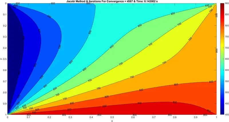
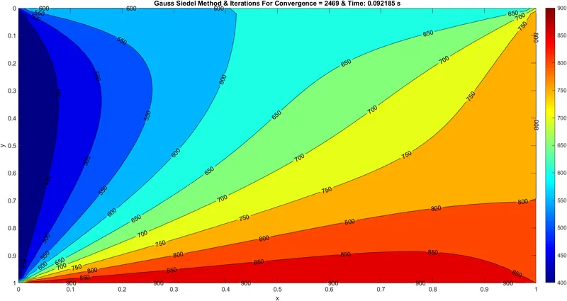
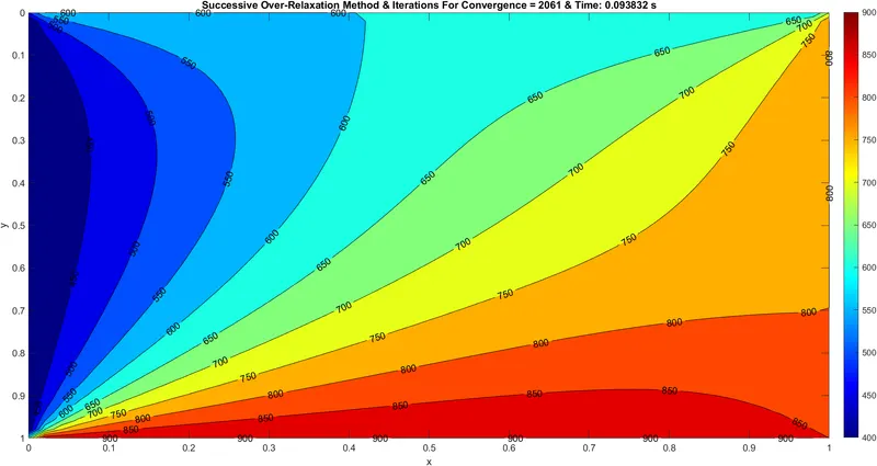
For transient state explicit case :

clear all
close all
clc
%% Inputs
L = 1;  %% Domain Length
nx = 50; %% Grid Points
ny=nx;
%�lculations 
x=linspace(0,L,nx);
dx=x(2)-x(1);
y=linspace(0,L,ny);
dy=y(2)-y(1);
%% Time Marching Step
t = 0.1;
nt = 1400;
dt = t/nt;
%% Coefficient Of Thermal Diffusion
alpha = 1.4; 
%�L Condition
CFL_x= alpha*dt/(dx)^2; 
CFL_y= alpha*dt/(dy)^2;
ct = 0;
%% Boundary Condition
T=300*ones(nx,ny);
T(:,1)= 400 ;   %% Left Wall
T(1,:)= 600;    %% Top Wall
T(:,end)= 800;  %% Right Wall
T(end,:)= 900;  %% Bottom Wall

T(1,1)= (400+600)/2 ; 
T(1,end)= (600+800)/2 ; 
T(end,1)= (400+900)/2 ; 
T(end,end)= (900+800)/2 ; 

Told = T;
k1 = (alpha*dt)/(dx^2);
k2 = (alpha*dt)/(dy^2);
%% Loop
tic
for k = 1:nt
    for i = 2:nx-1
        for j =2:ny-1
            H = (Told(i-1,j) - 2*Told(i,j) + Told(i+1,j));
            V = (Told(i,j+1) - 2*Told(i,j) + Told(i,j-1));
            T(i,j) = Told(i,j) + k1*H + k2*V;
        end
    end
    Told = T;
    ct = ct+1;
    time = toc;
end
%% Plotting
figure(1)
contourf(x,y,T,'ShowText','on');
colorbar
colormap(jet)
xlabel('x');
ylabel('y');
text = sprintf("Transient Explicit Heat Conduction Method & Iterations For Convergence = %d & Time: %f s",ct ,time);
title(text);
set(gca,'YDIR','reverse');

Output :

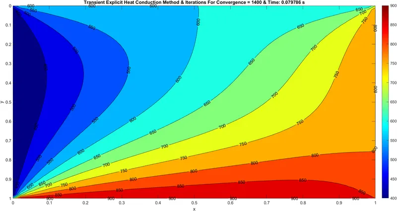
For Transient State Implicit Case :

 clear all
close all
clc
%% Inputs
L = 1; %% Domain Length
nx = 50; %% Grid Points
omega  = 1.1; %% Relaxation Factor
error = 9e9;  %% Error
tol = 1e-4;   %% Tolerance
alpha = 1.4;  %% Coefficient Of Thermal Diffusion
ct = 0;
ny=nx;
%% Time Marching Steps
t = 0.1; 
nt = 1400; 
dt = t/nt;
�lculations
x=linspace(0,L,nx);
dx=x(2)-x(1);
y=linspace(0,L,ny);
dy=y(2)-y(1);
%% Boundary Condition
T=300*ones(nx,ny);
T(:,1)= 400 ;   %% Left Wall
T(1,:)= 600;    %% Top Wall
T(:,end)= 800;  %% Right Wall
T(end,:)= 900;  %% Bottom Wall

T(1,1)= (400+600)/2 ; 
T(1,end)= (600+800)/2 ; 
T(end,1)= (400+900)/2 ; 
T(end,end)= (900+800)/2 ; 

Told = T;
T_prev = T;
k1 = (alpha*dt)/(dx^2);
k2 = (alpha*dt)/(dy^2);

%% Command Prompt For Choosing Iterative Solver
prompt = "Select Iterative Solver, Jacobi = 1, Gauss-Siedel = 2, SOR = 3  ";
iterative_solver = input(prompt);
%% Iterative Solution For Jacobi Method  
if iterative_solver == 1
    tic
    Jacobi = 1;
    for k = 1:nt
        error = 9e9;
        while(error>tol)
            for i = 2:nx-1
                for j =2:ny-1
                    term1 = 1/(1+2*k1+2*k2);
                    term2 = k1*term1;
                    term3 = k2*term1;
                    H = (Told(i-1,j) + Told(i+1,j));
                    V = (Told(i,j+1) + Told(i,j-1));            
                    T(i,j) = (term1*(T_prev(i,j)))+(term2*H)+(term3*V);
                end
            end
            error = max(max(abs(Told-T)));
            Told = T;
            ct = ct+1;
        end
        T_prev = T;
    end
    time = toc;
    %% Plotting
    figure(1)
    contourf(x,y,T,'ShowText','on')
    colorbar
    colormap(jet)
    xlabel('X-axis');
    ylabel('Y-axis');
    text = sprintf("Jacobi Method & Iterations For Convergence = %d & Time: %f s",ct ,time);
    title(text);
    set(gca,'YDIR','reverse');
end
%% Iterative Solution For Gauss Siedel Method
if iterative_solver == 2
    tic
    GS = 2;
    for k = 1:nt
        error = 9e9;
        while(error>tol)
            for i = 2:nx-1
                for j =2:ny-1
                    term1 = 1/(1+2*k1+2*k2);
                    term2 = k1*term1;
                    term3 = k2*term1;
                    H = (T(i-1,j) + Told(i+1,j));
                    V = (Told(i,j+1) + T(i,j-1));            
                    T(i,j) = (term1*(T_prev(i,j)))+(term2*H)+(term3*V);
                end
            end
            error = max(max(abs(Told-T)));
            Told = T;
            ct = ct+1;
        end
        T_prev = T;
    end
    time = toc;
    %% Plotting
    figure(2)
    contourf(x,y,T,'ShowText','on')
    colorbar
    colormap(jet)
    xlabel('X-axis');
    ylabel('Y-axis');
    text = sprintf("Gauss Siedel Method & Iterations For Convergence = %d & Time: %f s",ct ,time);
    title(text);
    set(gca,'YDIR','reverse');
end
%% Iterative Solution For Successive Over-Relaxation Method
if iterative_solver == 3
    tic
    SOR = 3;
    for k = 1:nt
        error = 9e9;
        while(error>tol)
            for i = 2:nx-1
                for j =2:ny-1
                    term1 = 1/(1+2*k1+2*k2);
                    term2 = k1*term1;
                    term3 = k2*term1;
                    H = (T(i-1,j) + Told(i+1,j));
                    V = (Told(i,j+1) + T(i,j-1));            
                    T(i,j) = (1-omega)*(Told(i,j)) + (omega*((term1*(T_prev(i,j)))+(term2*H)+(term3*V)));
                end
            end
            error = max(max(abs(Told-T)));
            Told = T;
            ct = ct+1;
        end
        T_prev = T;
    end
    time = toc;
    %% Plotting
    figure(3)
    contourf(x,y,T,'ShowText','on')
    colorbar
    colormap(jet)
    xlabel('X-axis');
    ylabel('Y-axis');
    text = sprintf("Successive Over-Relaxation Method & Iterations For Convergence = %d & Time: %f s",ct ,time);
    title(text);
    set(gca,'YDIR','reverse');
end

Output :

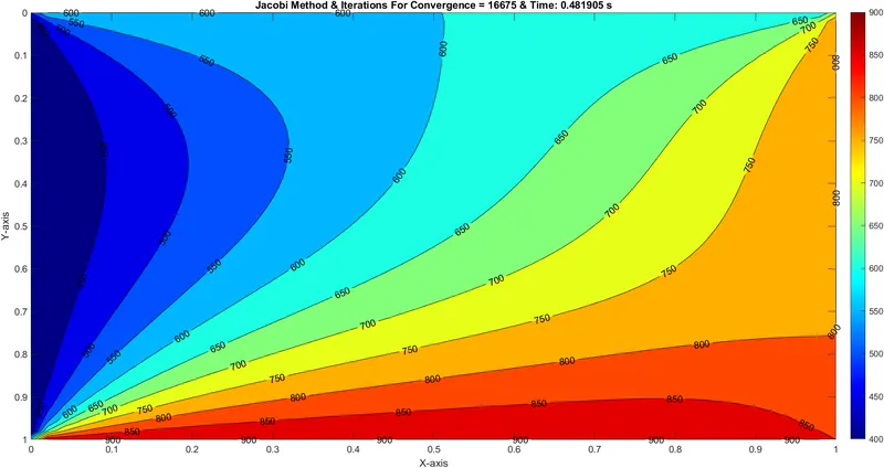
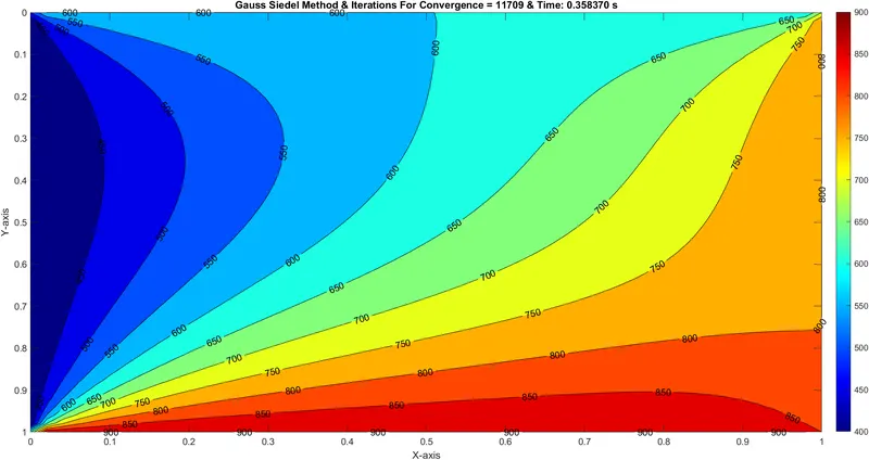
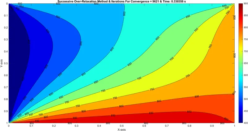
Compare the convergence rate [Number of iteration] of the steady state and transient [explicite and implicit] simulation and justify the numerics.

Method	Iteration for convergence	Time Taken TO Reach Convergence(seconds)
Jacobi method for steady state case	4587	0.140518
Gauss seidel method for steady state case	2469	0.087779
SOR for steady state case	2061	0.089496
Transient explicit method	1400	0.082067
Jacobi method forTransient case	16675	0.472450
Gauss seidel method for Transient case	11709	0.349222
SOR method for Transient case	9621	0.326980

Form the above analysis , we can conclude taht for steady case and transient implicit case the order of convergence is jacobi Method > Gauss siedel method > SOR method. Jacobi takes the most no of iteration and SOR method takes up the leadt no of iteration for reaching convergence.

Coeffecient of thermal diffusion can help us in attaining convergence faster but very hiigh co efficient of thermal diffusion values can also cause  divergence.

SOR method tries to extrapolate values of relaxation factor than SOR method also lead to divergence.

Transient explicit method is converging way faster than SOR method also as in explicit case CFL factore and coefficient of thermal diffusion comes into plys which is helping us in reaching convergence faster.