Week 5.1 - Mid term project - Solving the steady and unsteady 2D heat conduction problem

Aim: Solve the 2D heat conduction equation by using the point iterative techniques.

Objectives:

To solve the 2D heat conduction equation by using the point iterative techniques such as 

• Jacobi
• Gauss-seidel
• Successive over-relaxation

The Boundary conditions for the problem are as follows;

Top Boundary = 600 K

Bottom Boundary = 900 K

Left Boundary = 400 K

Right Boundary = 800 K

And, the absolute error criteria are 1e-4,

The following are the cases that the equation should solve;

1.  Steady state equation solving.
2. Unsteady state equation solving using explicit scheme.
3. Unsteady state equation solving using implicit scheme. 

Consider, that the area is a square geometry under the given boundary conditions

 Steady state equation solving:

In the steady state condition, the amount of heat that leaves a body is equal to the amount of heat entering body without varying with time.

The general, 2D steady state heat conduction equation with no heat generation is 

(δ²T)/(δx²)+(δ²T)/(δy²)=0

Discretization: Here, we use the central differencing method to discretize the second order PDE w.r.t x and y, that takes the information from both sides of the node.

so, by discretizing the above PDE using Central differencing scheme we get:

((T_L-2T_P+T_R)/(δx²) + ((T_T-2T_P+T_B)/(δy²))=0

By simplifying the above equation:

T_p  =1/K ((T_L+T_R)/(δx²) + (T_T+T_B)/(δy²))

where, K= 2*((δx²)+(δy²)/(δx²δy²)

The above equation can be solved to compute the Temperature distribution by using fixed points method like Jacobi, Gauss-seidel, Successive over-relaxation.

Jacobi Method:

Tⁿ⁺¹_i,j = 1/K (((Tⁿ_i-1,j +Tⁿ_{i+1, j})/δx²) + (Tⁿ_{i, j-1}+Tⁿ_i,j+1)/δy²)

Here, from this method the Temperature Tⁿ⁺¹_i,j is converged with Tⁿ by  n no.of iterating at each node repeatedly. After the equation is converged the Tⁿ value is updated with Tⁿ⁺¹_i,j This method is also called the method of simultaneous displacements.

Gauss Seidel:

Tⁿ⁺¹_i,j = 1/K (((Tⁿ⁺¹_i-1,j +Tⁿ_{i+1, j})/δx²) + (Tⁿ⁺¹_{i, j-1}+Tⁿ_i,j+1)/δy²)

Here, the Tⁿ⁺¹_i,j is converged with Tⁿ⁺¹ by  n+1 no.of iterating at each node repeatedly. Here we are solving the n+1th equation so the t old values are updated till nth iteration.

Successive over-relaxation:

Tⁿ⁺¹_i,j = Tⁿ_{i, j}(1-ω) + ω(T_G.S)

where ω is relaxation factor

if ω > 1 ⇒ over relaxation 

    ω<1>

Usually SOR is a enhance iterative method that enhancers the values of Gauss seidel

Matlab code:

Explanation:

• At first, we defined the input and boundary condition parameters of matrix T as 10x10 and defined the axis length as 1m and error as 1 and tolerance value as 1e-4
• And the above calculated K equation is defined and then calculated the corner points of the square matrix by taking the average of adjacent points.
• Here, we define the convergence loop and space loop then define the specified iteration equation as derived above, when we run the iteration, the maximum temperature is calculated within the tolerance.
• After the completion of the iteration the old values of T are updated.
• Then plotted the x, y and T values 

Results:

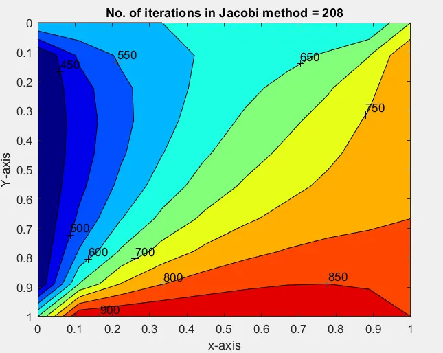
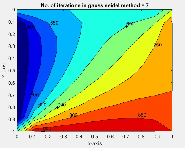
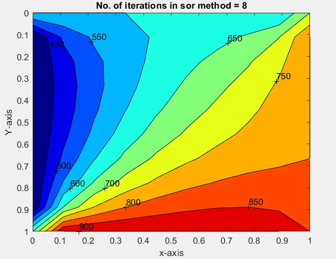
Conclusion:

Here, we observe that for all type of iterative techniques the results are almost similar and the plotted graph is similar in all cases, but the number iterations ran in the Jacobi method are more nearly 208 and the rest of the methods results less iterations.

Unsteady state (or) Transient state equation solving using explicit scheme:

In a transient state condition, the heat transfer takes place between the system and surroundings within the boundary condition by varying the time interval. Then general two-dimensional heat transfer equation in Transient state condition is:

(δT/δt)=α((δ²T)/(δx²)+(δ²T)/(δy²))

(Tⁿ⁺¹_p-Tⁿ_p)/Δt = α ((T_L-2T_P+T_R)/(∇x²) + ((T_T-2T_P+T_B)/(∇y²⁾)ⁿ 

If it runs n timesteps = explicit

if it runs n+1 timesteps = implicit

(Tⁿ⁺¹_p-Tⁿ_p)/Δt = Tⁿ_p+ K1(T_L-2T_P+T_R)ⁿ + K2(T_T-2T_P+T_B)ⁿ

where, CFL_x = K1 = (αΔt)/(∇x²))

            CFL_y = K2 = (αΔt)/(∇y²)

the solution is efficient if CFL_x + CFL_y  ≤ 0.5 and considering α =1.4

Matlab code:

clear all

close all

clc

<!-- [if mso]>
<![endif]-->

%inputs and boundary conditions

t_t = 600;

t_b = 900;

t_l = 400;

t_r = 800;

nx = 10;

ny = nx; % size of matrix

T=100*ones(nx,ny); %initial temperature 100k

x = linspace(0,1,nx);

y = linspace(0,1,ny);

dx=(x(2)-x(1));

dy=(y(2)-y(1));

tolerance = 1e-4;

alpha=1.4;

dt=1e-4;

<!-- [if mso]>
<![endif]-->

T(2:ny - 1, 1) = t_l; %first column elements

T(2:ny - 1, nx) = t_r; %last column elements

T(1, 2:nx - 1) = t_t; %first row elements

T(ny, 2:nx - 1) = t_b; %last row elements

%assigning the values at the corner positions of the T matrix by taking average of adjacent values

T(1,1)=(t_l+t_r)/2;

T(ny,1)=(t_l+t_b)/2;

T(1,nx)=(t_r+t_t)/2;

T(ny,nx)=(t_r+t_b)/2;

%solving the equation using explicit scheme

T_old = T;

term1=T;

term2=T;

term3=T;

error_expicit=1;

<!-- [if mso]>
<![endif]-->

%time loop

for nt=1:1400

error =1;

%convergence loop

while (error > tolerance)

%space loop

for i=2:nx-1

for j=2:ny-1

% simplified explicit equation

term1 = T_old(i,j);

term2= alpha*(dt/(dx^2))*((T_old(i+1,j)-2*T_old(i,j)+T_old(i-1,j)));

term3= alpha*(dt/(dy^2))*((T_old(i,j+1)-2*T_old(i,j)+T_old(i,j-1)));

T(i,j)=term1+term2+term3;

end

end

error = max(max(abs(T_old - T)));

T_old = T; % updating the old T values

error_expicit = error_expicit+1;

end

end

<!-- [if mso]>
<![endif]-->

contourf(x,y,T) -countour plot

clabel(contourf(T))

colormap(jet)

set(gca, 'ydir', 'reverse')

xlabel x-axis

ylabel y-axis

title(sprintf('No. of iterations in explict method = %d',error_expicit));

pause(1);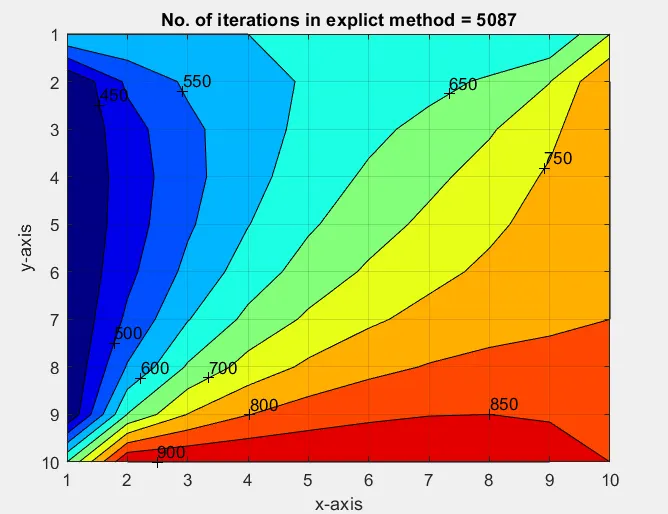

 

Results:

 

Here the solution is convergred at 5087th iteration.

 

Explanation:

• At first, we defined the inputs and boundary conditions of the matrix of size 10x10 that means it's a square matrix and calculated the corner mid points of the matrix.
• And defined the axis length as 1m and error as 1 and tolerance value as 1e-4, alpha value as 1.4. Then I defined the initial error and T old values.
• Then mentioned the time loop and convergence loop, then the space loop.
• Then, we defined the simplified explicit scheme by simplifying the terms. After the computation of the code loop vise within the tolerance limits.
• After that the T old values are updated at the end of the iterations.
• Then plotted the contour values of x and y and temperature T values in the graph.

 

Unsteady state (or) Transient state equation solving using Implicit scheme:

The genearl expression for the implicit scheme of  linear differential equation in a Trasient state condition of is stated as follows,

Tⁿ⁺¹_p  = ((1)/(1+2K₁+2K₂))*(Tⁿ_p)+K₁(T_L+T_R)ⁿ⁺¹+K₂(T_T+T_B)ⁿ⁺¹

This solution is solved by using the three scheme solvers i.e.., Jacobi, Gauss-seidel,SOR.

here let us consider the

Term_1 = (1+2K₁+2K₂)^-1 

Term_2 = K₁Term_1

Term_3 = K₂Term_1

And also consider H=T_old_(i-1,j)+T_old_(i+1,j) 

V= T_old_(i.j-1)+T_old_(i,j+1)

For Jacobi method:

T_(i,j)  = (T_prev_dt(i,j)*term_1)+(H*Term_2)+(v*Term_3)

For Gauss-seidel method:

T(i,j)= (Term_1*T_prev(i,j))+(Term_2*H)+(Term_3*V)

For Successive over relaxation:

T(i,j)=  (1-ω)*T(i,j) + ω*((Term_1*T_prev(i,j))+(Term_2*H)+(Term_3*V))

Matlab code:

clear all

close all

clc

<!-- [if mso]>
<![endif]-->

%inputs and boundary conditions

t_t = 600;

t_b = 900;

t_l = 400;

t_r = 800;

nx = 10;

ny = nx; % size of matrix

T=270*ones(nx,ny); %initial temperature 270k

x = linspace(0,0.1,nx);

y = linspace(0,0.1,ny);

dx=(x(2)-x(1));

dy=(y(2)-y(1));

tolerance = 1e-4;

error=1;

alpha=1.4;

dt=0.2;

T(2:ny - 1, 1) = t_l; %first column elements

T(2:ny - 1, nx) = t_r; %last column elements

T(1, 2:nx - 1) = t_t; %first row elements

T(ny, 2:nx - 1) = t_b; %last row elements

%assigning the values at the corner positions of the T matrix by taking average of adjacent values

T(1,1)=(t_l+t_r)/2;

T(ny,1)=(t_l+t_b)/2;

T(1,nx)=(t_r+t_t)/2;

T(ny,nx)=(t_r+t_b)/2;

<!-- [if mso]>
<![endif]-->

T_old = T;

T_prev =T;

k1=alpha*(dt/dx^2);

k2=alpha*(dt/dy^2);

term1=(1+(2*k1)+(2*k2))^-1;

term2=k1*term1;

term3=k2*term1;

w=1.4;

jacobi_method=1;

GS_method=1;

SOR_method=1;

jacobi_iter=1;

% Jacobi method

if (jacobi_method==1)

for nt=1:1400 % time loop

while error>tolerance % convergence loop

for i=2:nx-1 % space loop

for j=2:ny-1

H=(T_old(i-1,j)) + (T_old(i+1,j));

V=(T_old(i,j-1)) + (T_old(i,j+1));

T(i,j) = ((term1*T_prev(i,j)) + (term2*H) + (term3*V));

end

end

 

error=max(max(abs(T_old-T)));

T_old=T;

T_prev = T;

jacobi_iter=jacobi_iter+1;

end

 

figure(1)

contourf(x,y,T)

clabel(contourf(T))

colormap(jet)

set(gca, 'ydir', 'reverse')

xlabel x-axis

ylabel y-axis

title(sprintf('no.of iterations in Jacobi method = &d time steps = %d',jacobi_iter,nt))

pause(0.05)

end

end

% Gauss-seidel

GS_iter=1;

if (GS_method==1)

for nt=1:1400 % time loop

while error > tolerance % convergence loop

for i=2:nx-1 % space loop

for j=2:ny-1

H=(T_old(i-1,j)) + (T_old(i+1,j));

V=(T_old(i,j-1)) + (T_old(i,j+1));

T(i,j) = ((term1*T_prev(i,j)) + (term2*H) + (term3*V));

end

end

GS_iter=GS_iter+1;

error=max(max(abs(T_old-T)));

T_old=T;

T_prev = T_old;

end

<!-- [if mso]>
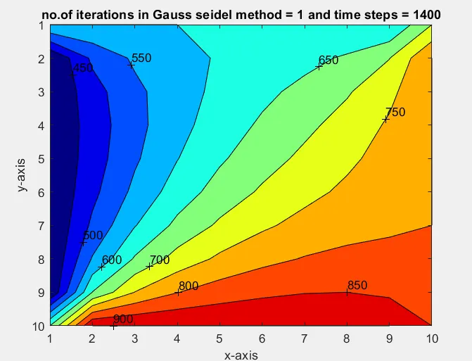
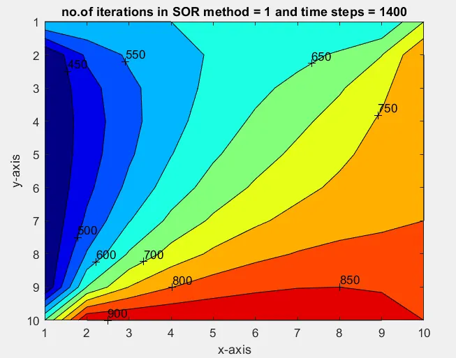
<![endif]-->

figure(2)

contourf(x,y,T)

clabel(contourf(T))

colormap(jet)

set(gca, 'ydir', 'reverse')

xlabel x-axis

ylabel y-axis

title(sprintf('no.of iterations in Gauss seidel method = %d time steps = %d',GS_iter,nt))

pause(0.03)

end

end

%Successive Over relaxation

SOR_iter = 1;

if (SOR_method==1)

for nt=1:1400 % time loop

while error > tolerance % convergence loop

for i=2:nx-1 % space loop

for j=2:ny-1

H=(T_old(i-1,j)) + (T_old(i+1,j));

V=(T_old(i,j-1)) + (T_old(i,j+1));

T(i,j) = (1-w)*T(i,j)+w*((term1*T_prev(i,j)) + (term2*H) + (term3*V));

end

 

end

SOR_iter=SOR_iter+1;

error=max(max(abs(T_old-T)));

T_old=T;

T_prev = T_old;

end

figure(3)

contourf(x,y,T)

clabel(contourf(T))

colormap(jet)

set(gca, 'ydir', 'reverse')

xlabel x-axis

ylabel y-axis

title(sprintf('no.of iterations in SOR method = %d time steps = %d',SOR_iter,nt))

pause(0.03)

end

end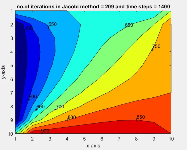

 

Results

 

Explanation:

• At first, we defined the inputs and boundary conditions of the matrix of size 10x10 that means it's a square matrix and calculated the corner mid points of the matrix.
• And defined the axis length as 1m and error as 1 and tolerance value as 1e-4, alpha value as 1.4. Then I defined the initial error and T old values.
• Then mentioned the time loop and convergence loop, then the space loop of all the three interative methods.
• After the computation of the code loop vise within the tolerance limits, and plotted the T, x and y coordinates by defining the no of iterations and tiimesteps.
• Her, after the end of iterations the iterative method and the Told valued are updated.

Conclusion:

Here, the equation is converged by using three interative methods and we observed that the Jacobi method run more iterative steps that other. 

The rate of iterations is Jacobi > Gauss-seidel > Successive over relaxation. 

In the Steady state condition the given equation is converged with less iterations and less time steps compared to Transient state stimulation. And by comparing both the stimulation methods Successive over relaxation method ran effectively with less iteratives for converging the equation in both Emplicit and Implicit schemes.