Challenge

Week 5.1 - Mid term project - Solving the steady and unsteady 2D heat conduction problem

SSumit Kamble16 Jul 2023

Aim:-

Steady state analysis & Transient State Analysis

1) To solve the 2D heat conduction equation by using the point iterative techniques.

The Boundary conditions for the problem are as follows;

Top Boundary = 600 K

Bottom Boundary = 900 K

Left Boundary = 400 K

Right Boundary = 800 K

we will implement the following methods for solving implicit equations.

Jacobi
Gauss-seidel
Successive over-relaxation

The absolute error criteria is 1e-4.

2. Write the code for both implicit and explicit schemes (This is for the transient analysis only)

3. Compare the convergence rate [Number of iterations] of the steady state and transient [explicit and implicit] simulations and justify the numerics.

Following are the inputs for the simulation.

- The computational area is unit square meter.

-Assume number of node points in x directions and number of nodes in y direction are same.

(we assume nx=ny=10)

-temperature at boundary is given.(boundary condition).

Top Boundary = 600 K

Bottom Boundary = 900 K

Left Boundary = 400 K

Right Boundary = 800 K

- At other location we initially assume temperature as 300K.

Theory:-

Heat transfer: Heat transfer is the science that seeks to predict the energy transfer that mey take place between material bodies as a result of temperature difference.

Conduction Heat transfer :- When temperature gradient exists in the body, there is an energy transfer from the high temperature region to the low temperature region. This energy is transferred by conduction and that the heat transfer rate per unit area is proportional to the normal temperature gradient.

There are two types of conduction heat transfer

a) Steady state heat conduction

b) Unsteady/ Tansient heat conduction

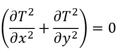
The two dimensional steady state heat conduction equation is given as,

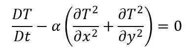
And The two dimensional unsteady state heat conduction equation is given as,

) Implicit Steady state 2D heat conduction equation solution.

A) Steady state heat conduction by using Jacobi Method:-

close all
clear all
clc

%Solving the Steady state 2D heat conduction by using Jacobi Method

%Input Parameters
%Number of grid points
%considering the unit square meter of domain.

nx = 10;
ny = nx; %same numbers of grid points in bothe directions.

x = linspace(0,1,nx);
y = linspace(0,1,ny);

dx = x(2) - x(1);
dy = dx;

%Absolute error criteria > tolerance
error = 9e9;
tolerance = 1e-4;

% Boundary conditions
T_L = 400;      %left side wall temperature
T_T = 600;      % top side wall temperature
T_R = 800;      % right side wall temperature
T_B = 900;      %bottom side wall temperature

T = 300*ones(nx,ny); % Assuming (initial guess) 300k temperature at all other points.

T(2:ny - 1, 1)  = T_L;
T(2:ny - 1, nx) = T_R;
T(1, 2:nx - 1)  = T_T;
T(ny, 2:nx - 1) = T_B;

%Calculating Average temperature at corners
T(1,1) = (T_T + T_L)/2;
T(nx,ny) = (T_R + T_B)/2;
T(1,ny) = (T_T + T_R)/2;
T(nx,1) = (T_L + T_B)/2;

%Assigning orginal values to T
T_intial = T;
T_old = T;


%Calculation of 2D steady state heat conduction equation by Jacobi method
iterative_solver = 1;

if iterative_solver == 1
    jacobi_iteration = 1;
    
    while(error > tolerance)
        
        for i = 2:nx - 1
            
            for j = 2:ny - 1
                T(i,j) = 0.25*(T_old(i-1,j) + T_old(i+1,j) + T_old(i,j-1) + T_old(i,j+1));
            end
            
        end
        
        error = max(max(abs(T_old - T)));
        T_old = T;
        jacobi_iteration = jacobi_iteration + 1;  
        
    end
end

%Plotting the graph which represents the temperature distribution over
%domain.
figure(1)
contourf(x,y,T)
clabel(contourf(x,y,T))
colorbar
colormap(jet)
set(gca, 'ydir', 'reverse')

xlabel('X-Axis')
ylabel('Y-Axis')
title(sprintf('No. of Jacobi Iterations(IMPLICIT) = %d', jacobi_iteration));
pause(0.03);

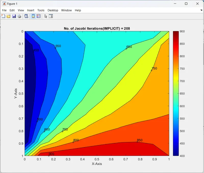
Output of Jacobi Method.

B) Steady state heat conduction by using Gauss Seidel Method:-

close all
clear all
clc

%Solving the Steady state 2D heat conduction by using gauss seidel Method

%Input Parameters
%Number of grid points
%considering the unit square meter of domain.

nx = 10;
ny = nx; %same numbers of grid points in bothe directions.

x = linspace(0,1,nx);
y = linspace(0,1,ny);

dx = x(2) - x(1);
dy = dx;

%Absolute error criteria > tolerance
error = 9e9;
tolerance = 1e-4;

% Boundary conditions
T_L = 400;      %left side wall temperature
T_T = 600;      % top side wall temperature
T_R = 800;      % right side wall temperature
T_B = 900;      %bottom side wall temperature

T = 300*ones(nx,ny); % Assuming (initial guess) 300k temperature at all other points.

T(2:ny - 1, 1)  = T_L;
T(2:ny - 1, nx) = T_R;
T(1, 2:nx - 1)  = T_T;
T(ny, 2:nx - 1) = T_B;

%Calculating Average temperature at corners
T(1,1) = (T_T + T_L)/2;
T(nx,ny) = (T_R + T_B)/2;
T(1,ny) = (T_T + T_R)/2;
T(nx,1) = (T_L + T_B)/2;

%Assigning orginal values to T
T_intial = T;
T_old = T;



%Calculation of 2D steady state heat conduction equation by Gauss-Seidel method
iterative_solver = 2;

if iterative_solver == 2
    Gauss_seidel_iteration = 1;
    
    while(error > tolerance)
        
        for i = 2:nx - 1
            
            for j = 2:ny - 1
                T(i,j) = 0.25*(T(i-1,j) + T_old(i+1,j) + T(i,j-1) + T_old(i,j+1));
            end
            
        end
        
        error = max(max(abs(T_old - T)));
        T_old = T;
        Gauss_seidel_iteration = Gauss_seidel_iteration + 1;  
        
    end
end

%Plotting the graph which represents the temperature distribution over
%domain.
figure(1)
contourf(x,y,T)
clabel(contourf(x,y,T))
colorbar
colormap(jet)
set(gca, 'ydir', 'reverse')

xlabel('X-Axis')
ylabel('Y-Axis')
title(sprintf('No. of Gauss-Seidel Iterations(IMPLICIT) = %d', Gauss_seidel_iteration));
pause(0.03);

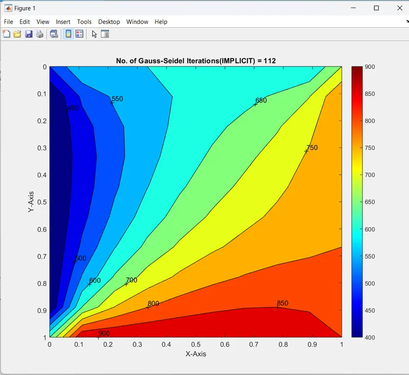
Output of Gauss- Seidel Method

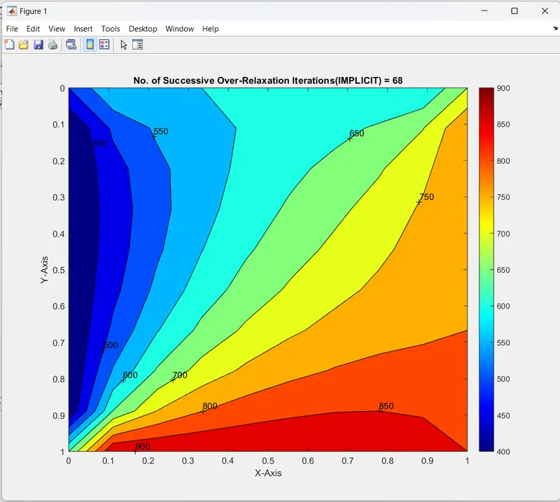
C) Steady state heat conduction by using Successive over relaxation Method:-

close all
clear all
clc

%Solving the Steady state 2D heat conduction (Successive over-relaxation Method)

%Input Parameters
%Number of grid points
%considering the unit square meter of domain.

nx = 10;
ny = nx; %same numbers of grid points in bothe directions.

x = linspace(0,1,nx);
y = linspace(0,1,ny);

dx = x(2) - x(1);
dy = dx;

%Absolute error criteria > tolerance
error = 9e9;
tolerance = 1e-4;
alpha=1.25;

% Boundary conditions
T_L = 400;      %left side wall temperature
T_T = 600;      % top side wall temperature
T_R = 800;      % right side wall temperature
T_B = 900;      %bottom side wall temperature

T = 300*ones(nx,ny); % Assuming (initial guess) 300k temperature at all other points.

T(2:ny - 1, 1)  = T_L;
T(2:ny - 1, nx) = T_R;
T(1, 2:nx - 1)  = T_T;
T(ny, 2:nx - 1) = T_B;

%Calculating Average temperature at corners
T(1,1) = (T_T + T_L)/2;
T(nx,ny) = (T_R + T_B)/2;
T(1,ny) = (T_T + T_R)/2;
T(nx,1) = (T_L + T_B)/2;

%Assigning orginal values to T
T_intial = T;
T_old = T;


%Calculation of 2D steady state heat conduction equation by Successive over-relaxation method
iterative_solver = 3;

if iterative_solver == 3
    Successive_Over_Relaxation_iteration = 1;
    
    while(error > tolerance)
        
        for i = 2:nx - 1
            
            for j = 2:ny - 1
                T(i,j) = alpha*(0.25*(T(i-1,j) + T_old(i+1,j) + T(i,j-1) + T_old(i,j+1))) + (1 - alpha)*T_old(i,j);
            end
            
        end
        
        error = max(max(abs(T_old - T)));
        T_old = T;
        Successive_Over_Relaxation_iteration = Successive_Over_Relaxation_iteration + 1;  
        
    end
end

%Plotting
figure(1)
contourf(x,y,T)
clabel(contourf(x,y,T))
colorbar
colormap(jet)
set(gca, 'ydir', 'reverse')

xlabel('X-Axis')
ylabel('Y-Axis')
title(sprintf('No. of Successive Over-Relaxation Iterations(IMPLICIT) = %d', Successive_Over_Relaxation_iteration));
pause(0.03);

Output of Successive over relaxation Method

2) Implicit Unsteady state 2D heat conduction equation solution.

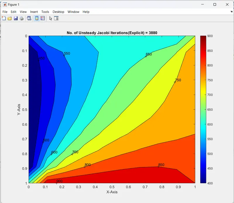
A) Unsteady state heat conduction by using Jacobi Method:-

close all
clear all
clc

%Solving the Unsteady state 2D heat conduction by Jacobi Method(IMPLICIT SCHEME)

%Input Parameters
%Number of grid points
%considering the unit square meter of domain.
nx = 10;
ny = nx;
nt = 1400;

x = linspace(0,1,nx);
y = linspace(0,1,ny);

dx = x(2) - x(1);
dy = dx;

%Absolute error criteria > tolerance
error = 9e9;
tolerance = 1e-4;
dt = 1e-3;

% Boundary conditions
T_L = 400;      %left side wall temperature
T_T = 600;      % top side wall temperature
T_R = 800;      % right side wall temperature
T_B = 900;      %bottom side wall temperature

T = 300*ones(nx,ny);

T(2:ny - 1, 1)  = T_L;
T(2:ny - 1, nx) = T_R;
T(1, 2:nx - 1)  = T_T;
T(ny, 2:nx - 1) = T_B;

%Calculating Average temperature at corners
T(1,1) = (T_T + T_L)/2;
T(nx,ny) = (T_R + T_B)/2;
T(1,ny) = (T_T + T_R)/2;
T(nx,1) = (T_L + T_B)/2;

%Assigning orginal values to T
T_old = T;
T_intial = T;

%Calculation of 2D steady heat conduction equation by Jacobi method
k1 = 1.1*(dt/(dx^2));
k2 = 1.1*(dt/(dy^2));

Jacobi_iteration = 1;
for k = 1:nt
    error = 9e9; 
    
    while(error > tolerance)
        
        for i = 2:nx - 1
            
            for j = 2:ny - 1
                    
                Term_1 = 1/(1 + (2*k1) + (2*k2));
                Term_2 = k1*Term_1;
                Term_3 = k2*Term_1;
                H = (T_old(i-1,j)) + (T_old(i+1,j));
                V = (T_old(i,j+1)) + (T_old(i,j-1));
                    
                T(i,j) = (T_intial(i,j)*Term_1) + (H*Term_2) + (V*Term_3);
   
            end
            
        end
        
        error = max(max(abs(T_old - T)));
        T_old = T;
        Jacobi_iteration = Jacobi_iteration + 1;  
               
    end
     T_intial = T;

    
%Plotting the graph which represents the temperature distribution over
%domain.
    figure(1)
    contourf(x,y,T)
    clabel(contourf(x,y,T))
    colorbar
    colormap(jet)
    set(gca, 'ydir', 'reverse')

    xlabel('X-Axis')
    ylabel('Y-Axis')
    title(sprintf('No. of Unsteady Jacobi Iterations(Explicit) = %d', Jacobi_iteration));
    pause(0.03)
end

Output of Jacobi Method.

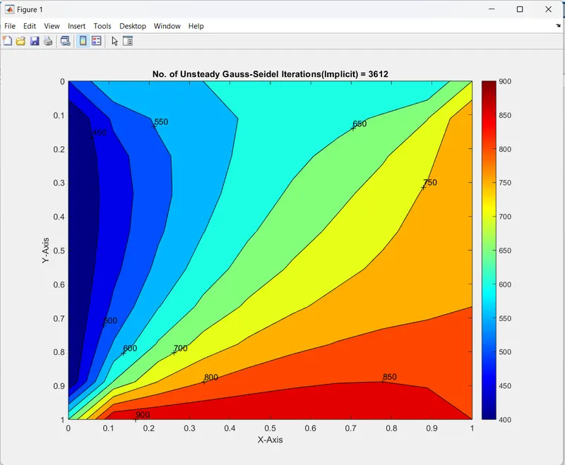
B) Unsteady state heat conduction by using Gauss- Seidel Method:-

close all
clear all
clc

%Solving the Unsteady state 2D heat conduction by Gauss Seidel Method(IMPLICIT SCHEME)

%Input Parameters
%Number of grid points
nx = 10;
ny = nx; %same numbers of grid points in bothe directions.
nt = 1400;

x = linspace(0,1,nx);
y = linspace(0,1,ny);

dx = x(2) - x(1);
dy = dx;

%Absolute error criteria > tolerance
error = 9e9;
tolerance = 1e-4;
dt = 1e-3;

% Boundary conditions
T_L = 400;      %left side wall temperature
T_T = 600;      % top side wall temperature
T_R = 800;      % right side wall temperature
T_B = 900;      %bottom side wall temperature

T = 300*ones(nx,ny); % Assuming (initial guess) 300k temperature at all other points.

T(2:ny - 1, 1)  = T_L;
T(2:ny - 1, nx) = T_R;
T(1, 2:nx - 1)  = T_T;
T(ny, 2:nx - 1) = T_B;

%Calculating Average temperature at corners
T(1,1) = (T_T + T_L)/2;
T(nx,ny) = (T_R + T_B)/2;
T(1,ny) = (T_T + T_R)/2;
T(nx,1) = (T_L + T_B)/2;

%Assigning orginal values to T
T_old = T;
T_intial = T;

%Calculation of 2D steady heat conduction equation by Gauss seidel method
k1 = 1.1*(dt/(dx^2));
k2 = 1.1*(dt/(dy^2));

Gauss_Seidel_iteration = 1;
for k = 1:nt
    error = 9e9; 
    
    while(error > tolerance)
        
        for i = 2:nx - 1
            
            for j = 2:ny - 1
                    
                Term_1 = 1/(1 + (2*k1) + (2*k2));
                Term_2 = k1*Term_1;
                Term_3 = k2*Term_1;
                H = (T(i-1,j)) + (T_old(i+1,j));
                V = (T(i,j+1)) + (T_old(i,j-1));
                    
                T(i,j) = (T_intial(i,j)*Term_1) + (H*Term_2) + (V*Term_3);
   
            end
            
        end
        
        error = max(max(abs(T_old - T)));
        T_old = T;
        Gauss_Seidel_iteration = Gauss_Seidel_iteration + 1;  
        
    end
    
    T_intial = T;
    
    %Plotting
    figure(1)
    contourf(x,y,T)
    clabel(contourf(x,y,T))
    colorbar
    colormap(jet)
    set(gca, 'ydir', 'reverse')

    xlabel('X-Axis')
    ylabel('Y-Axis')
    title(sprintf('No. of Unsteady Gauss-Seidel Iterations(Implicit) = %d', Gauss_Seidel_iteration));
    pause(0.03)
end

Output of Gauss- Seidel Method

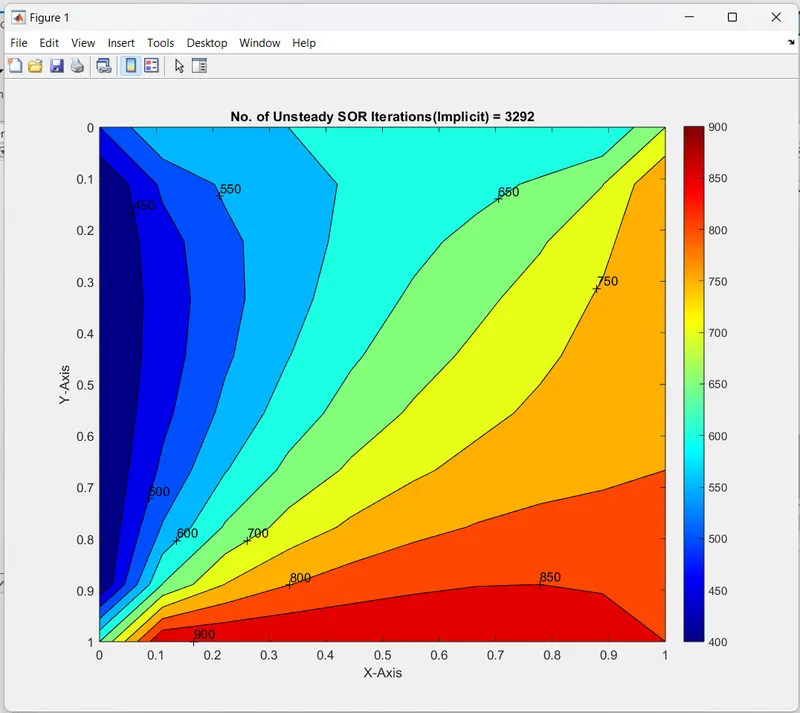
C) Unsteady state heat conduction by using successive over relaxation Method:-

close all
clear all
clc

%Solving the Unsteady state 2D heat conduction by Successive over-relaxation Method(IMPLICIT SCHEME)

%Input Parameters
%Number of grid points
nx = 10;
ny = nx; %same numbers of grid points in bothe directions.
nt = 1400;

x = linspace(0,1,nx);
y = linspace(0,1,ny);

dx = x(2) - x(1);
dy = dx;

%Absolute error criteria > tolerance
error = 9e9;
tolerance = 1e-4;
dt = 1e-3;
alpha = 1.25;

% Boundary conditions
T_L = 400;      %left side wall temperature
T_T = 600;      % top side wall temperature
T_R = 800;      % right side wall temperature
T_B = 900;      %bottom side wall temperature

T = 300*ones(nx,ny);

T(2:ny - 1, 1)  = T_L;
T(2:ny - 1, nx) = T_R;
T(1, 2:nx - 1)  = T_T;
T(ny, 2:nx - 1) = T_B;

%Calculating Average temperature at corners
T(1,1) = (T_T + T_L)/2;
T(nx,ny) = (T_R + T_B)/2;
T(1,ny) = (T_T + T_R)/2;
T(nx,1) = (T_L + T_B)/2;

%Assigning orginal values to T
T_old = T;
T_intial = T;
T_end = T;

%Calculation of 2D unsteady state heat conduction equation by Successive over-relaxation method
k1 = 1.1*(dt/(dx^2));
k2 = 1.1*(dt/(dy^2));

Successive_over_relaxation_iteration = 1;
for k = 1:nt
    error = 9e9; 
    
    while(error > tolerance)
        
        for i = 2:nx - 1
            
            for j = 2:ny - 1
                    
                Term_1 = 1/(1 + (2*k1) + (2*k2));
                Term_2 = k1*Term_1;
                Term_3 = k2*Term_1;
                H = (T(i-1,j)) + (T_old(i+1,j));
                V = (T(i,j+1)) + (T_old(i,j-1));
                    
                T(i,j) = (T_intial(i,j)*Term_1) + (H*Term_2) + (V*Term_3);
                T_end(i,j) = ((1-alpha)*T_old(i,j)) + (T(i,j)*alpha);
                
            end
            
        end
        
        error = max(max(abs(T_old - T)));
        T_old = T_end;
        Successive_over_relaxation_iteration = Successive_over_relaxation_iteration + 1;  
        
    end
    
    T_intial = T_end;
    
%Plotting the graph which represents the temperature distribution over
%domain.
    figure(1)
    contourf(x,y,T)
    clabel(contourf(x,y,T))
    colorbar
    colormap(jet)
    set(gca, 'ydir', 'reverse')

    xlabel('X-Axis')
    ylabel('Y-Axis')
    title(sprintf('No. of Unsteady SOR Iterations(Implicit) = %d', Successive_over_relaxation_iteration));
    pause(0.03)
end

Output of Successive over relaxation Method

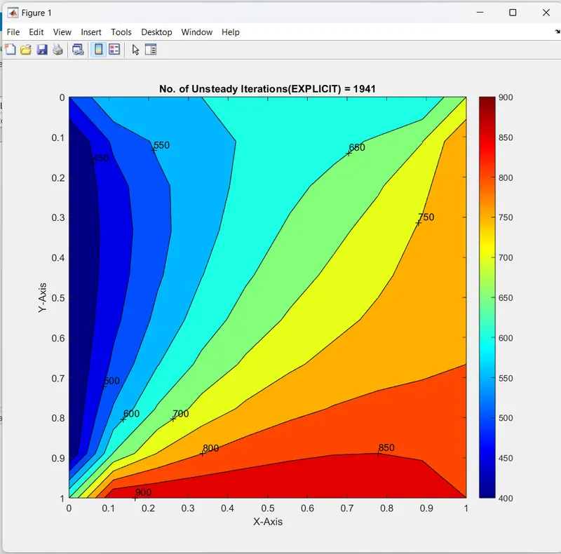
3) Explicit Unsteady state heat conduction by using Jacobi Method :-

close all
clear all
clc

%Solving the Unsteady state 2D heat conduction (EXPLICIT SCHEME)

%Input Parameters
%Number of grid points
nx = 10;
ny = nx;  %same numbers of grid points in bothe directions.
nt = 1400;

x = linspace(0,1,nx);
y = linspace(0,1,ny);

dx = x(2) - x(1);
dy = dx;

%Absolute error criteria > tolerance
error = 9e9;
tolerance = 1e-4;
dt = 1e-3;
omega = 1.1;

% Boundary conditions
T_L = 400;      %left side wall temperature
T_T = 600;      % top side wall temperature
T_R = 800;      % right side wall temperature
T_B = 900;      %bottom side wall temperature

T = 300*ones(nx,ny);

T(2:ny - 1, 1)  = T_L;
T(2:ny - 1, nx) = T_R;
T(1, 2:nx - 1)  = T_T;
T(ny, 2:nx - 1) = T_B;

%Calculating Average temperature at corners
T(1,1) = (T_T + T_L)/2;
T(nx,ny) = (T_R + T_B)/2;
T(1,ny) = (T_T + T_R)/2;
T(nx,1) = (T_L + T_B)/2;

%Assigning orginal values to T
T_intial = T;
T_old = T;


%Calculation of 2D unsteady heat conduction equation by Jacobi method
iterative_solver = 1;
k1 = 1.1*(dt/(dx^2));
k2 = 1.1*(dt/(dy^2));

if iterative_solver == 1
    Unsteady_Explicit = 1;
    for k = 1:nt
        error = 1; 
    
        while(error > tolerance)
        
            for i = 2:nx - 1
            
                for j = 2:ny - 1
                    Term_1 = T_old(i,j);
                    Term_2 = k1*(T_old(i+1,j) - 2*T_old(i,j) + (T_old(i-1,j)));
                    Term_3 = k2*(T_old(i,j+1) - 2*T_old(i,j) + T_old(i,j-1));
                    T(i,j) = Term_1 + Term_2 + Term_3;
                end
            
            end
        
            error = max(max(abs(T_old - T)));
            T_old = T;
            Unsteady_Explicit = Unsteady_Explicit + 1;  
        
        end
    end
end

%Plotting the graph which represents the temperature distribution over
%domain.
figure(1)
contourf(x,y,T)
clabel(contourf(x,y,T))
colorbar
colormap(jet)
set(gca, 'ydir', 'reverse')

xlabel('X-Axis')
ylabel('Y-Axis')
title(sprintf('No. of Unsteady Iterations(EXPLICIT) = %d', Unsteady_Explicit));
pause(0.03);

Output:

Conclusion:

a) From above program output and number of iteration required to converge the solution we can observed that

Jacobi method> Gauss- Seidel Method> Successive over-relaxation (required number of iteration)

b) The steady state equation required less numbers of iteration than unsteady/ transient eqaution for convergence.

c) From above programmes we will conclude that the successive over relaxation method converged solution more faster than other methods, in both implicit and explicit type.

Week 5.1 - Mid term project - Solving the steady and unsteady 2D heat conduction problem

Ship work like this
in your own course.

Talk to a career counsellor

Ship work like thisin your own course.

Talk to a career counsellor

Ship work like this
in your own course.