Week 5.1 - Mid term project - Solving the steady and unsteady 2D heat conduction problem

The 2D unsteady and steady state heat conduction equation is studied.

Unsteady State:

`(partial T)/(partial t) = alpha*((partial^2 T )/(partial x^2) + (partial^2 T )/(partial y^2) )`

Steady State:

`(partial^2 T )/(partial x^2) + (partial^2 T )/(partial y^2) = 0`

To evaluate the above equation for steady and unsteady state, iterative solvers are needed. The iterative solvers like Jacobi, Gauss-Seidel and Successive Over Relaxation are used. These equations are PDEs and they required numerical discretization techniques for analysis. In steady state analysis, numerical discretization is not required while in unsteady state analysis, equations can be solved either by explicit or implicit method.

Iterative Methods:

Jacobi Iterative Method is considered as an iterative algorithm to determine the solution for the system of linear equations. In it, an approximate value is used and then the entire equation is solved using the guess value, until the solution converges. In the jacobi method, the values of `T_i^n` obtained in the nth iteration remain unchanged until the entire (n+1)th iteration has been calculated.

In Gauss-Seidel Method the new values of `T_i^(n+1)` are used as soon as they are known. The difference between Gauss-Seidel and Jacobi method is that the Jacobi method uses the value obtained from the previous step while the Gauss-Seidel method always applies the latest updated values during the iterative procedures.

The Successive Over Relaxation Method uses a value of omega to guess the value for the next iteration. By employing the below mentioned formula the values are computed.

`T_i^(n+1) = (1 - omega)* T_i^n + omega * TGS`

In this TGS is the value computed using the Gauss-Seidel iteration method formula. The Gauss-Seidel method is extended to the relaxation methods.

For unsteady state analysis, the implicit and explicit scheme are defined as follows:

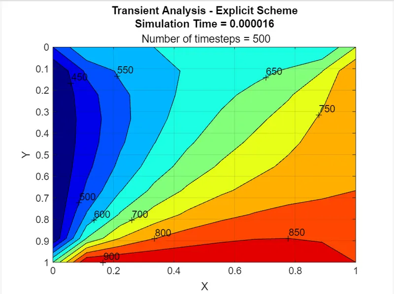
Explicit: As RHS is completely known the iterative solvers are not required. The temperature at each node is calculated directly. The only parameter to be kept in check is the CFL indicated as in the program. The summation of both should be less than or equal to 0.5 for the analysis to be stable.

`T_p^(n+1) = T_p^n + k_1*(T_L - 2*T_p + T_R)^n + k_2*(T_B - 2*T_p + T_T)^n`

Implicit: The RHS of the equation are unknown, the iterative solvers are required to evaluate the temperature function. The three iterative methods discussed above are used.

`T_p^(n+1) = (1/(1 + 2*k_1 + 2*k_2))*[T_p^n + k_1*(T_L + T_R)^(n+1) + k_2*(T_B + T_T)^(n+1)]`

The above equation is simplified further and implemented in Matlab.

% Steady-State Analysis
clear all
close all
clc
% Input
nx = 10; % Number of Nodes in X direction
ny = 10; % Number of Nodes in Y direction
dt = 1e-2; % Time Step
alpha = 1.4; % Thermal Diffusivity
% Defining Initial Conditions -
T = 300*ones(nx,ny); % Temperature Initial Guess
for i = 1:nx 
    T(1,i) = 600; % Top Boundary
    T(ny,i) = 900; % Bottom Boundary
end
for j = 1:ny
    T(j,1) = 400; % Left Boundary
    T(j,nx) = 800; % Right Boundary
end
% Corner Nodes - Boundary Conditions
T(1,1) = (T(1,2) + T(2,1))/2;
T(1,nx) = (T(1,nx-1) + T(2,nx))/2;
T(ny,1) = (T(ny-1,1) + T(ny,2))/2;
T(ny,nx) = (T(ny,nx-1) + T(ny-1,nx))/2;
% To create 2D Mesh 
x = linspace(0,1,nx);
y = linspace(0,1,ny);
dx = x(2) - x(1);
dy = y(2) - y(1);
% told = t
T_old=T;
error = 100;
tol = 1e-4;
k = 2*(dx^2+dy^2)/(dx^2*dy^2);
method = input('Iterative method = '); %iterative method selection
%JACOBI ITERATIVE METHOD
if (method==1)
    tic;
    jacobi = 1;
    while(error>tol)
        for i = 2:nx-1
            for j = 2:ny-1
                T(i,j) = (((T_old(i-1,j) + T_old(i+1,j))/(dx^2)) + ...
                ((T_old(i,j+1) + T_old(i,j-1))/(dy^2)))/k;
                %term_1 = ((T_old(i-1,j) + T_old(i+1,j))/(dx^2));
                %term_2 = ((T_old(i,j-1) + T_old(i,j+1))/(dy^2));
                %T(i,j) = (term_1 + term_2)/k;
            end
        end
 error = max(max(abs(T-T_old)));
 T_old = T;
 jacobi = jacobi+1;
 time_taken = toc;
    end
figure(1)
colormap(jet);
A = contourf(x,y,T);
clabel(A);
set(gca,'YDir','reverse');
xlabel('X')
ylabel('Y')
text1 = sprintf('Number of Iteration = %d', jacobi);
text2 = sprintf('Simulation Time = %f', time_taken);
title({'Steady State Heat Condustion profile by Jacobi'; text1; text2});
end
%GAUSS-SEIDEL ITERATIVE METHOD
if (method==2)
    tic;
    gauss = 1;
    while(error>tol)
        for i = 2:nx-1
            for j = 2:ny-1
            %term_1 = (T(i-1,j) + T_old(i+1,j))/(dx^2);
            %term_2 = (T_old(i,j+1) + T(i,j-1))/(dy^2);
            %T(i,j) = (term_1 + term_2)/k;
 
            T(i,j) = (((T(i-1,j) + T_old(i+1,j))/(dx^2))+ ...
            ((T_old(i,j+1) + T(i,j-1))/(dy^2)))/k;
            end
        end
 error = max(max(abs(T-T_old)));
 T_old = T;
 gauss = gauss+1;
 time_taken = toc;
    end
%plotting
figure(2)
colormap(jet);
A = contourf(x,y,T);
clabel(A);
set(gca,'YDir','reverse');
xlabel('X')
ylabel('Y')
text1 = sprintf('Number of Iteration = %d', gauss);
text2 = sprintf('Simulation Time = %f', time_taken);
title({'Steady State Heat Condustion profile by Gauss-Seidel'; text1; text2});
end
%SUCCESSIVE OVER RELAXATION ITERATIVE METHOD
if (method==3)
    tic;
    sor = 1;
    omega = 1.4; %over relaxation factor
    while(error>tol)
        for i = 2:nx-1
            for j = 2:ny-1
                term1 = (T(i-1,j) + T_old(i+1,j))/(dx^2);
                term2 = (T_old(i,j+1) + T(i,j-1))/(dy^2);
                T(i,j) = ((T_old(i,j)*(1-omega))) + (omega*(term1+term2))/k;
            end
        end
 error = max(max(abs(T-T_old)));
 T_old = T;
 sor = sor+1;
 time_taken = toc;
    end
%plotting
figure(3)
colormap(jet);
A = contourf(x,y,T);
clabel(A);
set(gca,'YDir','reverse');
xlabel('X')
ylabel('Y')
text1 = sprintf('Number of Iteration = %d', sor);
text2 = sprintf('Simulation Time = %f', time_taken);
title({'Steady State Heat Condustion profile by Successive Over Relaxation'; text1; text2});
end

% Unsteady State Analysis - Explicit Scheme
clear all
close all
clc
% Input
nx = 10; % Number of Nodes in X direction
ny = 10; % Number of Nodes in Y direction
dt = 0.002; % Time Step
alpha = 1.4; % Thermal Diffusivity
nt = 500; % Number of timesteps
% Defining Initial Conditions -
T = 300*ones(nx,ny); % Temperature Initial Guess
for i = 1:nx 
    T(1,i) = 600; % Top Boundary
    T(ny,i) = 900; % Bottom Boundary
end
for j = 1:ny
    T(j,1) = 400; % Left Boundary
    T(j,nx) = 800; % Right Boundary
end
% Corner Nodes - Boundary Conditions
T(1,1) = (T(1,2) + T(2,1))/2;
T(1,nx) = (T(1,nx-1) + T(2,nx))/2;
T(ny,1) = (T(ny-1,1) + T(ny,2))/2;
T(ny,nx) = (T(ny,nx-1) + T(ny-1,nx))/2;
% To create 2D Mesh 
x = linspace(0,1,nx);
y = linspace(0,1,ny);
dx = x(2) - x(1);
dy = y(2) - y(1);
T_old = T; % Initiating Temperature Value
k1 = alpha*(dt/(dx^2)); % Constant
k2 = alpha*(dt/(dy^2)); % Constant
CFL = k1 + k2; % CFL Value for Stability
for k = 1:nt % Time Loop
    tic;
    for i = 2:nx-1 % X direction
        for j = 2:ny-1 % Y direction
            T(i,j) = (T_old(i,j)+k1*(T_old(i+1,j)-2*T_old(i,j)+T_old(i-1,j))+k2*(T_old(i,j+1)-2*T_old(i,j)+T_old(i,j-1)));
        end
    end
 T_old = T; % updating previous values
 time_taken = toc;
 % Plot the T values
 figure(1)
 colormap(jet);
 A = contourf(x,y,T);
 clabel(A);
 set(gca,'YDir','reverse');
 xlabel('X');
 ylabel('Y');
 grid on;
 %text1 = sprintf('Number of Iteration = %d', sor);
 text2 = sprintf('Simulation Time = %f', time_taken);
 title({'Transient Analysis - Explicit Scheme'; text2});
 B = sprintf(' Number of timesteps = %d',k);
 subtitle(B);
 pause(0.0001);
end

% Unsteady State Analysis - Implicit Scheme
clear all
close all
clc
% Input
nx = 10; % Number of Nodes in X direction
ny = 10; % Number of Nodes in Y direction
dt = 0.01; % Time Step
alpha = 0.3; % Thermal Diffusivity
nt = 300; % Number of time steps
% Defining Initial Conditions -
T = 300*ones(nx,ny); % Temperature Initial Guess
for i = 1:nx 
    T(1,i) = 600; % Top Boundary
    T(ny,i) = 900; % Bottom Boundary
end
for j = 1:ny
    T(j,1) = 400; % Left Boundary
    T(j,nx) = 800; % Right Boundary
end
% Corner Nodes - Boundary Conditions
T(1,1) = (T(1,2) + T(2,1))/2;
T(1,nx) = (T(1,nx-1) + T(2,nx))/2;
T(ny,1) = (T(ny-1,1) + T(ny,2))/2;
T(ny,nx) = (T(ny,nx-1) + T(ny-1,nx))/2;
% To create 2D Mesh 
x = linspace(0,1,nx);
y = linspace(0,1,ny);
dx = x(2) - x(1);
dy = y(2) - y(1);
T_old=T; % t_old = t
T_prev_dt = T_old; % tprev_dt = t_old
tol = 1e-4;
k1 = alpha*dt/(dx^2);
k2 = alpha*dt/(dy^2);
method = input('Iterative method = '); %iterative method selection
%JACOBI ITERATIVE METHOD
if (method==1)
    tic;
    jacobi = 1;
    for z = 1:nt
        error = 100;
        while(error>tol)
            for i = 2:nx-1
                for j = 2:ny-1
                    term_1 = (1 + (2*k1) + (2*k2))^-1;
                    term_2 = k1*term_1;
                    term_3 = k2*term_1;
                    H = (T_old(i-1,j) + T_old(i+1,j));
                    V = (T_old(i,j-1) + T_old(i,j+1));
                    T(i,j) = (T_prev_dt(i,j)*term_1) + (H*term_2) + (V*term_3);
                end
            end
            error = max(max(abs(T-T_old)));
            T_old = T;
            jacobi = jacobi+1;
        end
    T_prev_dt = T;
    end
 time_taken = toc;
 
 % Plot
figure(1)
colormap(jet);
A = contourf(x,y,T);
clabel(A);
set(gca,'YDir','reverse');
xlabel('X')
ylabel('Y')
text1 = sprintf('Number of Iteration = %d', jacobi);
text2 = sprintf('Simulation Time = %f', time_taken);
title({'Steady State Heat Condustion profile by Jacobi'; text1; text2});
end
method = input('Iterative method = '); %iterative method selection
%JACOBI ITERATIVE METHOD
if (method==2)
    tic;
    gs = 1;
    for z = 1:nt
        error = 100;
        while(error>tol)
            for i = 2:nx-1
                for j = 2:ny-1
                    term_1 = (1 + (2*k1) + (2*k2))^-1;
                    term_2 = k1*term_1;
                    term_3 = k2*term_1;
                    H = (T(i-1,j) + T_old(i+1,j));
                    V = (T_old(i,j-1) + T(i,j+1));
                    T(i,j) = (T_prev_dt(i,j)*term_1) + (H*term_2) + (V*term_3);
                end
            end
        error = max(max(abs(T-T_old)));
        T_old = T;
        gs = gs+1;
        end
    T_prev_dt = T;
    end
 time_taken = toc;
 
 % Plot
figure(2)
colormap(jet);
A = contourf(x,y,T);
clabel(A);
set(gca,'YDir','reverse');
xlabel('X')
ylabel('Y')
text1 = sprintf('Number of Iteration = %d', gs);
text2 = sprintf('Simulation Time = %f', time_taken);
title({'Steady State Heat Condustion profile by Gauss Seidel'; text1; text2});
end
%SOR ITERATIVE METHOD
if (method==3)
    tic;
    sor = 1;
    omega = 1.2; % Over Relaxation Factor
    for z = 1:nt
        error = 100;
        while(error>tol)
            for i = 2:nx-1
                for j = 2:ny-1
                    term_1 = (1 + (2*k1) + (2*k2))^-1;
                    term_2 = k1*term_1;
                    term_3 = k2*term_1;
                    H = (T(i-1,j) + T_old(i+1,j));
                    V = (T_old(i,j+1) + T(i,j-1));
                    TGS = (T_prev_dt(i,j)*term_1) + (H*term_2) + (V*term_3);
                    T(i,j) = (((1-omega)*T_old(i,j)) + (omega*TGS));
                end
            end
        error = max(max(abs(T-T_old)));
        T_old = T;
        sor = sor+1;
        end
    T_prev_dt = T;
    end
 time_taken = toc;
 
 % Plot
figure(3)
colormap(jet);
A = contourf(x,y,T);
clabel(A);
set(gca,'YDir','reverse');
xlabel('X')
ylabel('Y')
text1 = sprintf('Number of Iteration = %d', sor);
text2 = sprintf('Simulation Time = %f', time_taken);
title({'Unsteady State Heat Condustion Profile by Successive Over Relaxation'; text1; text2});
end

Results:

For Steady State:-

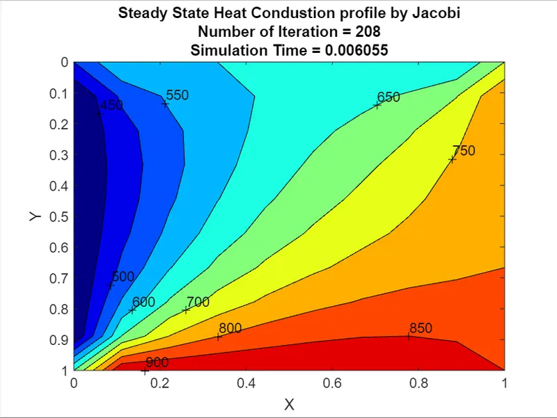
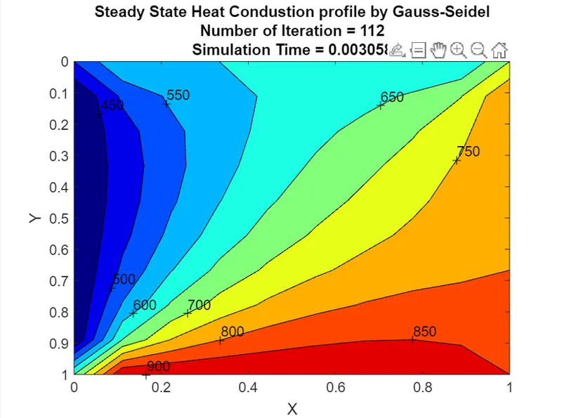
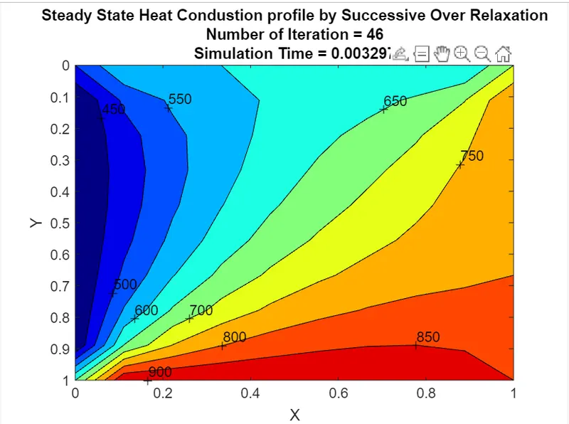
For Unsteady State - Explicit method:-

Unsteady State - Implicit:-

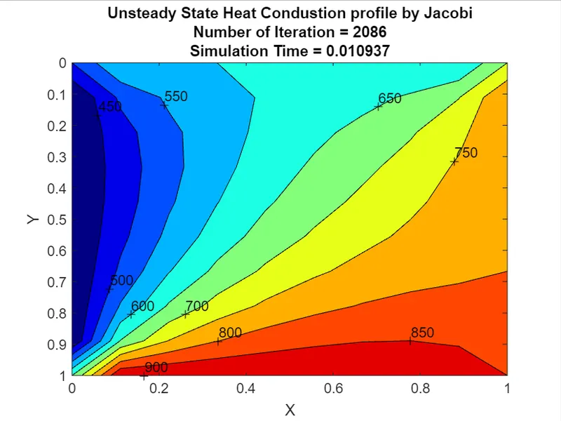
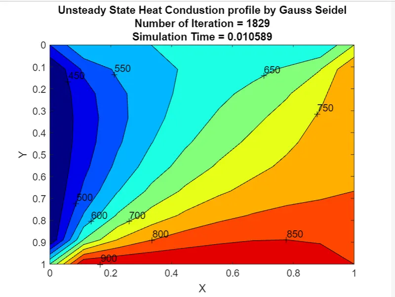
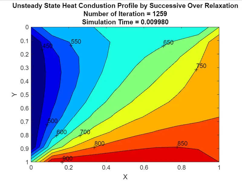
The following table shows the number of iterations taken by steady and unsteady state for different iterative methods.

Iterative Method	Steady State Analysis	Unsteady State Analysis
Explicit Scheme	N/A	500
Jacobi Method	208	2086
Gauss-Seidel Method	112	1555
Successive Over Relaxation	46	1259

Conclusion

The fastest steady state simulation versus fastest unsteady state simulation results have been compared.It was observed that on solving the steady and unsteady 2D heat conduction problem by using various iterative techniques like Jacobi, Gauss-Seidel and Successive Over Relaxation(SOR) methods, the Successive OverRelaxation method has shown the fastest convergence rate. The number of iteration required is least in SOR method and maximum in Jacobi method for both steady and unsteady state. So, the trend in terms of the number of iterations for convergence is the Jacobi method > Gauss-Seidel method > SOR method. The simulations are compared for different analysis methods, it was observed that in steady state analysis, the terms of thermal diffusivity (alpha) and time derivative (dt) are not included, resulting in a faster steady state simulation when compared to unsteady state analysis. The exact correlated values of dx & dy values give the accurate results. In unsteady state analysis, for the explicit method, time taken for convergence is very less and easy to solve. Here we have only a system of equations which are solved independently without iterations. This scheme is almost similar to the steady state analysis. The time integration is the convergence loop for the steady state case. In solving iterative methods, thermal diffusivity (alpha) and relaxation factor (omega) in SOR plays a keen role for an accurate and convergent simulation. Also, nodal size and time step plays a vital role for convergence. Therefore, in the steady state analysis and unsteady state analysis, SOR has the fastest convergence with a smaller number of iterations. We conclude that steady state SOR method does not include the thermal diffusivity and time derivative term which results in steady state solution, whereas for unsteady state SOR method it takes more time and high iterations to reach the steady state condition.