Week 3 - Solving second order ODEs

% Challenge 6 - ODE Solver function for simulation of motion of simple pendulum
function [dtheta_dt] = ODE_Damper_solver(t,theta,b,g,l,m)
% theta in radians
theta1 = theta(1);
theta2 = theta(2);
dtheta1_dt = theta2;
dtheta2_dt = -(b/m)*theta2-(g/l)*sin(theta1);
dtheta_dt = [dtheta1_dt;dtheta2_dt];
end

% Challenge 6 - Simulation of motion of simple pendulum
% Damping constant - Unitless
b = input("Enter the Damping constant:");
% Gravitational constant - m/(s)^2
g = 9.81;
% Length of pendulum in m
l = input("Enter length of Pendulum:");
% Mass of pendulum bob in kg
m = input("Enter mass of Pendulum Bob:");
theta_0 = input("Enter initial conditions in [ ]:");
% Time span in seconds
a = input("Initial time point:");
c = input("Final time point:");
n = input("No. of Intervals:");
time_span = linspace(a,c,n);
[t,results] = ode45(@(t,theta) ODE_Damper_solver(t, theta, b,g,l,m),time_span, theta_0);
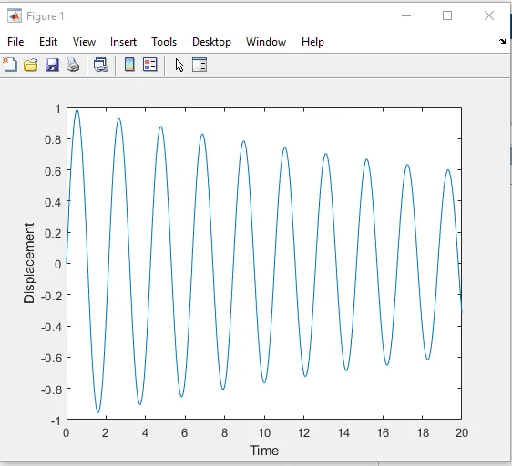
figure(1)
title('Displacement Vs Time plot')
plot(t,results(:,1))
xlabel('Time')
ylabel('Displacement')
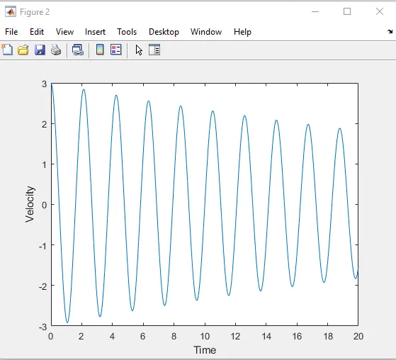
figure(2)
title('Velocity Vs Time plot')
plot(t,results(:,2))
xlabel('Time')
ylabel('Velocity')
figure(3)
title('Parameter Variation w.r.t. Time plot')
plot(t,results(:,1))
hold on
plot (t,results(:,2))
xlabel('Time')
ylabel('Parameters')
legend('Displacement','Velocity')
theta = results(:,1);
ct = 1;
for i = 1:length(theta)
    angle = theta(i);
    figure(4)
    title('Simple Penedulum animation')
    x0 = 0;
    y0 = 0;
    x1 = l*cos(((3*pi)/2)+angle);
    y1 = l*sin(((3*pi)/2)+angle);
    plot([x0 x1],[y0 y1],'linewidth',4)
    hold on
    plot(x1,y1,'.','markers',50)
    hold on
    plot([-5,5],[0,0],'linewidth',5)
    hold off
    axis([-9,9,-4,4])
    pause(0.09)
    G(ct) = getframe(gcf)
    ct = ct+1;
end
movie(G)
VideoFile = VideoWriter('Pendulum Animation.avi','Uncompressed AVI');
open(VideoFile)
writeVideo(VideoFile,G)
close(VideoFile)

TASK 1 - Coding the ODE solver function

1. By using the 'function' command, declare the variables that would be used in obtaining the values and the plot required for obtaining the simulation of the motion of the pendulum.
2. Type the expressions defining the derivative terms of the differential equation by assuming theta as theta1 and theta2 as the first order differential of theta1.
3. Type the obtained theta1 and theta2 into a column matrix.
4. Type 'end' command and save the file as ODE_Damper_solver.m

TASK 2 - Coding the solver to obtain values required for the Time variation plot

1. Type the values of the inputs required to solve the second order differential equation and obtain the values required to plot the variation plots
2. Use the 'ode45' command to solve the equation by declaring the variaboles of the equation and by calling the function saved from task 1.

TASK 3 - Plotting the Time variation plot

1. By using the 'plot' command, obtain the displacement vs time plot by typing the plot for theta1.
2. By using the 'plot' command, obtain the velocity vs time plot by typing the plot for theta2.
3. By using the 'plot' command, obtain the displacement and velocity vs time plot by typing the plot for theta1, 'hold on' command, and typing the plot for theta2 .
4. Input the legend in the 3rd plot by using 'legend' command.

TASK 4 - Simulating the motion of the pendulum

1. Since we require the simulation of motion (displacement) of the pendulum, equate a variable - theta - to the results of displacement used in plotting the first plot
2. Initiate a counter 'ct' by equating it to 1.
3. Initiate a 'for' loop describing the conditions required for obtaining the displacement plot.
4. Describe the initial x and y coordinates as 0
5. Type the expressions with which the next x and y coordinates (x1,y1) are calculated.
6. Plot the obtained x and y coordinates by using the 'plot' command and keeing the inewidth as 4.
7. Give the 'hold on' command and plot (x1, y1) by using 'plot' command, givein asterisk marker.
8. Give the range of the axes along with linewidt and type 'hold off' command.
9. Give a pause time of 0.09 and declare a variacle G(ct) equal to the getframe command.
10. Give an increment to the counter every time a frame is generated till the final frame.
11. Give the 'end' command. Type the movie command as 'movie(G)'. Use the 'VideoWriter' command to generate the videofile by giving the name of the file and the file type of the generated video.
12. Use 'open' command to open the video file, 'writeVideo' command to save it in the same location as the MATLAB program and 'close' command to close the video file.

ERRORS ENCOUNTERED:

The movie wasn't generated after the execution of the program because a required variable was missing information necessary to generate frames for simulating the motion of the pendulum.

MEASURES TAKEN TO RECTIFY THE ERRORS:

The required information for the variable was assigned, resulting in the generation of the frames required for simulating the motion of the pendulum.

RESULTS:

Link for Pendulum Animation