Project 2 - Rankine cycle Simulator

% Challenge 10 - Rankine Cycle
disp('Rankine Cycle');
disp('1-2 is isentropic expansion in turbine');
disp('2-3 is constant pressure heat removal in condenser');
disp('3-4 is isentropic compression in pump');
disp('4-1 is constant pressure heat addition in boiler');
% Inputs to be given
p1 = input('P1(in bar):');
t1 = input('T1(in celsius):');
p2 = input('P2(in bar):');
% Extracting data 
% State 1
h1 = XSteam('h_pT',p1,t1);
s1 = XSteam('s_pT', p1,t1);
% State 2
s2 = s1;
sf2 = XSteam('sL_p',p2);
sg2 = XSteam('sV_p',p2);
x2 = (s2-sf2)/(sg2-sf2);
hf2 = XSteam('hl_p',p2);
hg2 = XSteam('hV_p',p2);
h2 = hf2 + (x2*(hg2-hf2));
% State 3
p3 = p2;
s3 = XSteam('sL_p',p3);
h3 = XSteam('hL_p',p3);
% State 4
s4 = s3;
p4 = p1;
% Turbine Work
W_T = h1-h2;
v3 = XSteam('vL_p',p3);
% Pump Work
W_P = v3*(p4-p3)*100;
h4 = h3+W_P;
% Net Work
W_net = W_T-W_P;
Q_in = h1-h4;
Q_out = h2-h3;
% Thermal Efficiency
Thermal_eff = (W_net/Q_in)*100;
%Specific Steam Consumption
Sp_Steam_Consumption = (3600/W_net);
% Temperatures at state points
t3 = XSteam('Tsat_p',p3);
t2 = t3;
Cp4 = XSteam('Cp_ps',p4,s4);
Cv4 = XSteam('Cv_ps',p4,s4);
k = Cp4/Cv4;
t4 = t3/((p3/p4)^((k-1)/k));
% Temperature, entropy and enthalpy at the vapour and liquid line for
% plotting
t6 = XSteam('Tsat_p',p1);
s5 = XSteam('sL_p',p1);
s6 = XSteam('sV_p',p1);
h5 = XSteam('hL_p',p1);
h6 = XSteam('hV_p',p1);
t5 = t6;
% Plotting the Saturation Curve
t = linspace(1,375,1000);
for i = 1:length(t)
    sf(i) = XSteam('sL_t',t(i));
    sg(i) = XSteam('sV_t',t(i));
    hf(i) = XSteam('hL_t',t(i));
    hg(i) = XSteam('hV_t',t(i));
end
% T-S diagram
figure(1)
grid on
hold on
plot(sf,t,'r','linewidth',1)
plot(sg,t,'r','linewidth',1)
plot([s1 s2],[t1 t2],'k','linewidth',2)
plot([s2 s3],[t2 t3],'k','linewidth',2)
plot([s3 s4],[t3 t4],'k','linewidth',2)
plot([s4 s5],[t4 t5],'k','linewidth',2)
plot([s5 s6],[t5 t6],'k','linewidth',2)
s_c1 = linspace(s6,s1,1000);
for l = 1:length(s_c1)
    t_c1(l) = XSteam('t_ps',p1,s_c1(l));
end
plot(s_c1,t_c1,'k','linewidth',5)
text(s1+0.1,t1,'1')
text(s2+0.1,t2,'2')
text(s3,t3-20,'3')
text(s4,t4+20,'4')
title('Temperature vs Entropy')
xlabel('Entropy S(KJ/Kg.K)')
ylabel('Temperature T(degree C)')
legend('Saturation Curve','location','northwest')
% H-S diagram
figure(2)
grid on
hold on
plot(sf,hf,'g','linewidth',1)
plot(sg,hg,'g','linewidth',1)
plot([s1 s2],[h1 h2],'k','linewidth',2)
plot([s2 s3],[h2 h3],'k','linewidth',2)
plot([s3 s4],[h3 h4],'k','linewidth',2)
h_c = linspace(h4,h5,200);
for k = 1:length(h_c)
    sch(k) = XSteam('h_ps',p1,h_c(k));
end
plot(sch,h_c,'k','linewidth',5)
plot([s5 s6],[h5 h6],'k','linewidth',5)
for m = 1:length(s_c1)
    h_c1(m) = XSteam('h_ps',p1,s_c1(m));
end
plot(s_c1,h_c1,'k','linewidth',5)
text(s1+0.1,h1,'1')
text(s2+0.1,h2,'2')
text(s3,h3-100,'3')
text(s4,h4+200,'4')
title('Enthalpy vs Entropy')
xlabel('Entropy S(KJ/Kg.K)')
ylabel('Enthalpy H(KJ/Kg)')
legend('Saturation Curve','location','northwest')
% Displaying Results
disp('RESULTS')
fprintf('At State Point 1:\n');
fprintf('P1: %8.3f bar\n', p1);
fprintf('T1: %8.3f C\n', t1);
fprintf('H1: %8.3f KJ/Kg\n', h1);
fprintf('S1: %8.3f KJ/Kg.K\n', s1);
fprintf('At State Point 2:\n');
fprintf('P2: %8.3f barn', p2);
fprintf('T2: %8.3f C\n', t2);
fprintf('H2: %8.3f KJ/Kg\n', h2);
fprintf('S2: %8.3f KJ/Kg.K\n', s2);
fprintf('x2: %8.3f\n', x2);
fprintf('At State Point 3:\n');
fprintf('P3: %8.3f bar\n', p3);
fprintf('T3: %8.3f C\n', t3);
fprintf('H3: %8.3f KJ/Kg\n', h3);
fprintf('S3: %8.3f KJ/Kg.K\n', s3);
fprintf('At State Point 4:\n');
fprintf('P4: %8.3f bar\n', p4);
fprintf('T4: %8.3f C\n', t4);
fprintf('H4: %8.3f KJ/Kg\n', h4);
fprintf('S4: %8.3f KJ/Kg.K\n', s4);
fprintf('Turbine Work: %8.3f KJ/Kg\n', W_T);
fprintf('Pump Work: %8.3f KJ/Kg\n', W_P);
fprintf('Net. Work done: %8.3f KJ/Kg\n', W_net);
fprintf('Thermal Efficiency: %8.3f Percent\n', Thermal_eff);
fprintf('Specific Steam Consumption: %8.3f KJ/KWh', Sp_Steam_Consumption);

CODING THE RANKINE CYCLE SIMULATOR:

1. Display the steps involved in Rankine cycle - What sort of process each step is, by using the 'disp' command.
2. Give the pressure and temperature at the first stage and the pressure at second point by using input command.
3. Extract the Enthalpy and Entropy for all stages from the 'XSteam.m' file by calling the 'XSteam' function and give the relations between temperatures of each stage and pressures at each stage wherever required.
4. Calculate the Turbine Work, Pump Work, Net Work, Thermal Efficiency, Specific Steam Consumption.
5. Obtain Cp and Cv at stage 4 and Temperatures, Entropies and Enthalpies at the liquid and vapour lines from 'XSteam.m' file by calling the 'XSteam' command for plotting the same.
6. Obtain the points to plot the Saturation curve by using 'linspace' command and by extracting the required Enthalpy and Entropy data at given temperatures by using a 'for' loop to plot the points
7. Plot the T-S diagram by initiating the 'plot' command, using the data obtained for temperature and entropy from the 'XSteam.m' file and the calculations done in the above steps.
8. Obtain a dataset of 200 equally spaced values in between the entropies of the 6th and 1st stage by usig the 'linspace' and equate it to the variable 's_c1'.
9. Initiate a 'for' loop and give the conditions to obtain the values required to plot the T-S diagram. Equate the obtained values to the variable 't_c1'. Plot the obtained 's_c1', 't_c1' in the same plot as the above obtained T-S diagram by using 'hold on' command. Give the legend for saturation curve by using the 'legend' command, giving the location of the legend as north west.
10. Plot the H-S diagram by using the data obtained for enthalpy and entropy from the 'XSteam.m' file and the calculations done in the above steps.
11. Obtain a dataset of 200 equally spaced values in between the enthalpies of the 4th and 5th stage by using the 'linspace' command and equate it to the variable 'h_c'.
12. Initiate a 'for' loop and give the conditions to obtain the values required to plot the H-S diagram. Equate the obtained values to the variable 'h_c1'. Plot the obtained 's_c1', 'h_c1' in the same plot as the above obtained H-S diagram by using 'hold on' command. Give the legend for saturation curve by using the 'legend' command, giving the location of the legend as north west.
13. Display the results obtained by using the 'fprintf' command, giving the FormatSpec as '%8.3f' (floating point value of 8spaces and an accuracy of upto 3 decimal points).

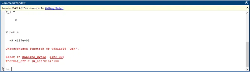
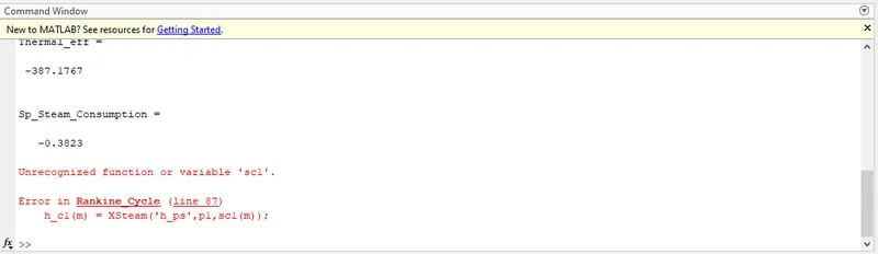
ERRORS OBTAINED:

Unrecognized variables obtained on running the code.

STEPS TAKEN TO RECTIFY THE ERRORS :

Changed the names of the variables in the code to their correctly assigned names, resulting in the errors being rsolved and the code giving the desired output.

RESULTS

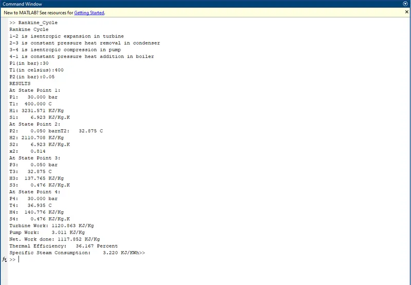
Resultsof the given Rankine Cycle problem

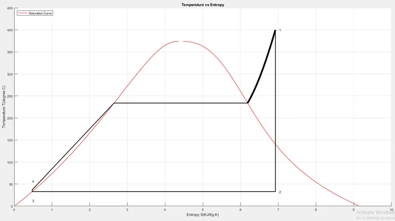
T-S Diagram of the given Rankine Cycle problem

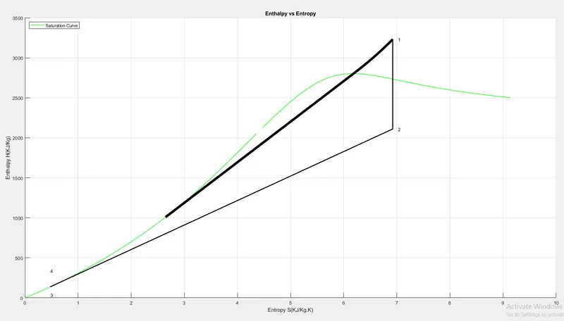
H-S Diagram of the given Rankine Cycle problem