Week 5.1 - Mid term project - Solving the steady and unsteady 2D heat conduction problem

The Steady and Unsteady 2D Heat Conduction Problem

Aim of this project is to analyse the effect of different iterative solvers for solving 2D heat conduction problem.

This problem demands to find the temperature distribution over a 2D sheet on steady and unsteady condition using different iterative solvers. The initial temperatures over 4 edges are given. First step is to simulate steady and undteady conditions of heat conduction using explicit and implicit method and then, compare the convergence rate & number of iterations of different iterative solvers used in implicit method.

Steady state condition

The condition when temperature at each point on the surface of 2D sheet is not varying with respect to time.

Explicit

In explicit condition the set of linear equations at a stage (timestep) are not coupled with the equation of another stage (timestep) so that they can be solved easily (analytically) without using iterative solvers. But here in steady state, explicit scheme is not suitable. Because for explicit we need to calculate the point at a particular time step from the data (values) obtained from previous time steps. But in steady state governing equation (1) there is no time derivative in governing equation which means there is no previous time steps.

Implicit

In implicit condition the set of linear equations at a stage (timestep) are coupled with the equation of another stage (timestep) so that we must assume the solutions initially then using iterative solvers, set of equations can be solved numerically.

Governing equation

`del^2/(delx^2) T+del^2/(dely^2) T=0`___________________eqn(1)

The above equation is an elliptic profile, so we need to make it discrete linear equations.

For convenience the governing equation in partial differential equation form is converted into linear algebraic equation.

`T_(i,j)= (∆x^2 ∆y^2)/(2(∆x^2+∆y^2))*[(T_(i-1,j)+T_(i+1,j))/(∆x^2 )+(T_(i,j-1)+T_(i,j+1))/(∆y^2 )]`

Simplifying,

`k= (2(∆x^2+∆y^2))/(∆x^2 ∆y^2)`

Discretized linear equation

`T_(i,j)^(n+1)= 1/k*[(T_(i-1,j)^n+T_(i+1,j)^n)/(∆x^2 )+(T_(i,j-1)^n+T_(i,j+1)^n)/(∆y^2 )]`

The iterative solvers are,

• Jacobi

In Jacobi method the input values of a particular iteration are obtained from the solution of previous iteration. The iterative values won’t get updated within an iteration. Following line of code shows the changes for Jacobi method, The left (i-1,j) , right (i+1,j) and top (i,j-1) , bottom ((i,j-1) points are all taken from T_old which is denoted as the previous iteration. Following is a line of code for steady state Jacobi method

` T_jac(i,j) = term*((T_oldj(i-1,j)+T_oldj(i+1,j))/(dx^2)+(T_oldj(i,j-1)+T_oldj(i,j+1))/(dy^2))`

• Gauss-seidel

Following code shows the changes for a steady state Gauss-seidel method, In the left (i-1,j) & bottom ((i,j-1) points, the values are taken from the current iteration T_g . Whereas the in top (i,j-1) & right (i+1,j) points, the values are same from T_old which is the previous iteration.

• As the values are updated within an iteration,
• This method gives a faster converging with lesser number of iterations

` Tg(i,j) = term*((Tg(i-1,j)+T_oldg(i+1,j))/dx^2 + (Tg(i,j-1)+T_oldg(i,j+1))/dy^2`

• Successive over-relaxation (SOR)

The following is a line of code for a steady state SOR method

`Ts(i,j) = term*((Ts(i-1,j)+T_olds(i+1,j))/dx^2 + (Ts(i,j-1)+T_olds(i,j+1))/dy^2);`

` Ts(i,j) = T_olds(i,j)*(1-omega)+(omega*Ts(i,j));`

• This method uses a relaxation factor (omega) for faster convergence

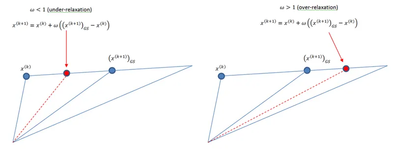
The successive over-relaxation (SOR) method is another form of the Gauss-Seidel method in which the new estimate at iteration k+1 for the component is calculated as the weighted average of the previous estimate and the estimate using Gauss-Seidel left

where can be obtained using the Gauss-Seidel method. The weight factor omega is chosen such that 0< omega < 2. If omega=1, then the method is exactly the Gauss-Seidel method. Otherwise, to understand the effect of omega we will rearrange the above equation to;

If 0<omega<1, then, the method gives a new estimate that lies somewhere between the old estimate and the Gauss-Seidel estimate, in this case, the algorithm is termed: “under-relaxation” (Figure 1). Under-relaxation can be used to help establish convergence if the method is diverging. If 1<omega<2, then the new estimate lies on the extension of the vector joining the old estimate and the Gauss-Seidel estimate and hence the algorithm is termed: “over-relaxation” (Figure 1). Over-relaxation can be used to speed up convergence of a slow-converging process. The following code defines and uses the SOR procedure to calculate the new estimates. Compare with the Gauss-Seidel procedure shown above.

Figure 1

Code for Steady Implicit

clear all
close all
clc

%Parameters
L = 1;
nx = 100;
ny = nx;

x = linspace(0,L,nx);
dx = x(2)-x(1);
y = linspace(0,L,ny);
dy = y(2)-y(1);
[XX, YY] = meshgrid(x, y);
%Temperature matrix jacobi
T_jac = 300*ones(ny,nx);
T_jac(:,1) = 400;
T_jac(1,:) = 600;
T_jac(:,end) = 800;
T_jac(end,:) = 900;
T_jac(1,1)=(600+400)/2;
T_jac(1,100)=(600+800)/2;
T_jac(100,100)=(900+800)/2;
T_jac(100,1)=(400+900)/2;
T_oldj = T_jac;
%Temperature matrix gaus seidel
Tg = 300*ones(ny,nx);
Tg(:,1) = 400;
Tg(1,:) = 600;
Tg(:,end) = 800;
Tg(end,:) = 900;
Tg(1,1)=(600+400)/2; %Corner nodes
Tg(1,100)=(600+800)/2;%Corner nodes
Tg(100,100)=(900+800)/2;%Corner nodes
Tg(100,1)=(400+900)/2;%Corner nodes
T_oldg=Tg;
%Temperature matrix succesive over relaxation
Ts = 300*ones(ny,nx);
Ts(:,1) = 400;
Ts(1,:) = 600;
Ts(:,end) = 800;
Ts(end,:) = 900;T_jac(1,1)=(600+400)/2; %Corner nodes
Ts(1,100)=(600+800)/2;%Corner nodes
Ts(100,100)=(900+800)/2;%Corner nodes
Ts(100,1)=(400+900)/2;%Corner nodes
T_olds=Ts;

term = (dx^2*dy^2)/(2*(dx^2+dy^2));

tol = 1e-4;
error = 100;

iteration_method = 1;%Iteration_method = 1-Jacobi ; 2-Gauss seidel ; 3-SOR
tic
if iteration_method == 1 %Jacobi method

    iter_jac = 0;%To start counting iteration
   
    while (error > tol)
        for j = 2:ny-1
            for i = 2:nx-1
                T_jac(i,j) = term*((T_oldj(i-1,j)+T_oldj(i+1,j))/(dx^2)+(T_oldj(i,j-1)+T_oldj(i,j+1))/(dy^2));
            end
        end
        error = max(max(abs(T_jac-T_oldj))); % max(max is taken to get the maximum of x and y coordinate.
        T_oldj = T_jac;
        iter_jac = iter_jac+1;%counting iteration
    end
 
end
   time_jac = toc;
   
iteration_method=2;
tic
if iteration_method == 2 %Gauss Seidel method
    iter_gas = 0;
    tol =1e-04;
    error =9e9;
    while (error > tol)
        for j = 2:ny-1
            for i = 2:nx-1
                Tg(i,j) = term*((Tg(i-1,j)+T_oldg(i+1,j))/dx^2 + (Tg(i,j-1)+T_oldg(i,j+1))/dy^2);
            end
        end
error = max(max(abs(Tg-T_oldg)));
T_oldg = Tg;
iter_gas = iter_gas+1;
    end
end
    
 time_gas = toc;
 
    iteration_method=3;
    tic
if iteration_method == 3 %SOR method
    omega = 1.8;
    error =9e9;
    iter_sor = 0;
    while (error > tol)
        for j = 2:ny-1
            for i = 2:nx-1
                Ts(i,j) = term*((Ts(i-1,j)+T_olds(i+1,j))/dx^2 + (Ts(i,j-1)+T_olds(i,j+1))/dy^2);
                Ts(i,j) = T_olds(i,j)*(1-omega)+(omega*Ts(i,j));
            end
        end
        error = max(max(abs(Ts-T_olds)));
        T_olds = Ts;
        iter_sor = iter_sor+1;
    end

end
   time_sor = toc;
    
%Plotting temperature contour on X and Y axes
figure(1);

contourf(XX,YY,T_jac)
ax.YDir = 'reverse';
colorbar
xlabel('X-axis')
ylabel('Y-axis')
title({'Steady state temperature profile';['Iteration Method = ',num2str(1)];['No. of iterations = ',num2str(iter_jac)];['Simulation time = ',num2str(time_jac),' s']})
grid on

figure(2);
contourf(XX,YY,Tg)
ax.YDir = 'reverse';
colorbar
xlabel('X-axis')
ylabel('Y-axis')
title({'Steady state temperature profile';['Iteration Method = ',num2str(2)];['No. of iterations = ',num2str(iter_gas)];['Simulation time = ',num2str(time_gas),' s']})
grid on

figure(3);
contourf (XX,YY,Ts);
ax.YDir = 'reverse';
colorbar
xlabel('X-axis')
ylabel('Y-axis')
title({'Steady state temperature profile';['Iteration Method = ',num2str(3)];['No. of iterations = ',num2str(iter_sor)];['Simulation time = ',num2str(time_sor),' s']})
grid on

Results-Steady State Implicit

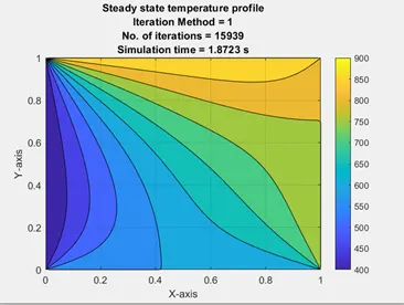
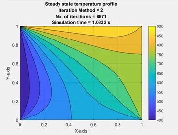
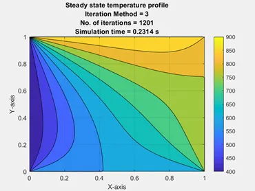
Observation: Number of Iterations for Jacobi>Gauss-seidel>Successive over-relaxation

Iterative time for Jacobi>Gauss-seidel>Successive over-relaxation

Transient state condition

The condition when temperature at each point on the surface of 2D sheet is varying at a particular rate until it reaches equilibrium (or steady state).

Explicit

Governing equation

`(delT)/(delt)=alpha((del^2T)/(delx^2) + (del^2T)/(dely^2))` ___________________eqn(2)

Discretized linear equation

k1 = alpha*dt/dx^2

k2 = alpha*dt/dy^2

`T(i,j)^(n+1)=T(i,j)^n+k1(T(i-1,j)^n-2(T(i,j)^n)+T(i+1,j)^n+k2(T(i,j+1)^n-2(T(i,j)^n)+T(i,j-1)^n))`

`T_(i,j)^(n+1) = T_(i,j)^n*[1-2*k_1-2*k_2] + k_1*(T_(i-1,j)^n + T_(i+1,j)^n) + k_2*(T_(i,j+1)^n + T_(i,j-1)^n) `

Code for Transient Explicit

clear all

close all

clc

 

%Parameters

L = 1;

nx = 100;

ny = nx;

dt = .14;

t = 1000;

nt = t/dt;

alpha = 1.75e-4;

 

x = linspace(0,L,nx);

dx = x(2)-x(1);

y = linspace(0,L,ny);

dy = y(2)-y(1);

CFL = alpha*dt*((1/dx^2)+(1/dy^2));

 

%Guess temperature matrix

T = 300*ones(ny,nx);

T(:,1) = 400;

T(1,:) = 600;

T(:,end) = 800;

T(end,:) = 900;

T(1,1)=(600+400)/2;

T(100,100)=(900+800)/2;

T(1,100)=(900+400)/2;

T(100,1)=(600+800)/2;

T_old = T;

 

k1 = alpha*dt/dx^2;

k2 = alpha*dt/dy^2;

 

iter = 0;

tic

%Time loop

for k = 1:nt

    %Y-Space loop

    for j = 2:nx-1

        %X-Space loop

        for i = 2:ny-1

            H = (T_old(i-1,j)-2*T_old(i,j)+T_old(i+1,j));

            V = (T_old(i,j-1)-2*T_old(i,j)+T_old(i,j+1));

            T(i,j) = T_old(i,j)+(H*k1)+(V*k2);

        end

    end

T_old = T;

iter = iter+1; %To count iteration

end

time = toc;

 

%Plotting temperature contour on X and Y axes

[c,h] = contourf(x,y,T);

colorbar

 

xlabel('X')

ylabel('Y')

title({'Transient state-Explicit temperature profile';['No. of iterations = ',num2str(iter),'    Time = ',num2str(t),' s'];['CFL = ',num2str(CFL),'     Simulation time = ',num2str(time)]})

grid on

Result-Transient Explicit

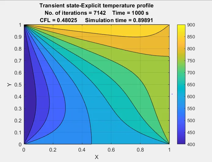
Observation: Solution is ustable if CFL is less than or equal to 0.5.

Implicit

In implicit condition the set of linear equations at a stage (timestep) are coupled with the equation of another stage (timestep) so that we must assume the solutions initially then using iterative solvers, set of equations can be solved numerically.

Governing equation

`(delT)/(delt)=alpha((del^2T)/(delx^2) + (del^2T)/(dely^2))`

Discretized linear equation

k1 = alpha*dt/dx^2

k2 = alpha*dt/dy^2

`T(i,j)^(n+1)=T(i,j)^n+k1(T(i+1,j)^(n+1)-2T(i,j)^(n+1)+T(i-1,j)^(n+1))+k2(T(i,j+1)^(n+1)-2T(i,j)^(n+1)+T(i,j+1)^(n+1))`

`T_(i,j)^(n+1) =( T_(i,j)^n + k_1*(T_(i-1,j)^(n+1) + T_(i+1,j)^(n+1)) + k_2*(T_(i,j+1)^(n+1) + T_(i,j-1)^(n+1)))/(1+2*k_1+2*k_2)`

The iterative solvers are,

• Jacobi

Following code shows the changes for transient state Jacobi method, The left (i-1,j) , right (i+1,j) and top (i,j-1) , bottom ((i,j-1) points are all taken from T_old which is denoted as the previous iteration.

k1 = alpha*dt/dx^2

k2 = alpha*dt/dy^2

term1 = 1/(1+2*k1+2*k2);

term2 = k1*term1;

term3 = k2*term1;

H = (T_oldg(i-1,j)+T_oldg(i+1,j));

V = (T_oldg(i,j-1)+T_oldg(i,j+1));

T_g(i,j) = (T_prevg(i,j)*term1)+(H*term2)+(V*term3);

• Gauss-seidel

Following code shows the changes for transient state Gauss-seidel method, In the left (i-1,j) & bottom ((i,j-1) points, the values are taken from the current iteration T_g whereas the top (i,j-1) & right (i+1,j) points, the values are same from T_old which is the previous iteration.

• As the values are updated within an iteration,
• This method gives a faster converging with lesser number of iterations

k1 = alpha*dt/dx^2

k2 = alpha*dt/dy^2

term1 = 1/(1+2*k1+2*k2);

term2 = k1*term1;

term3 = k2*term1;

H = (T_j(i-1,j)+T_oldj(i+1,j));

V = (T_j(i,j-1)+T_oldj(i,j+1));

T_j(i,j) = (T_prevj(i,j)*term1)+(H*term2)+(V*term3);

• Successive over-relaxation
• This method uses a relaxation factor (omega) for faster convergence

. Following are the lines of code for transient state Jacobi method;

term1 = 1/(1+2*k1+2*k2);

term2 = k1*term1;

term3 = k2*term1;

H = (Ts(i-1,j)+T_olds(i+1,j));

V = (Ts(i,j-1)+T_olds(i,j+1));

Ts(i,j) = (T_prevs(i,j)*term1)+(H*term2)+(V*term3);

Ts(i,j) = T_olds(i,j)*(1-omega)+omega*Ts(i,j);

Here T_prevs is previous time step value and T_olds is previous iteration value.

Code for Transient Implicit

clear all
close all
clc

%Parameters
L = 1;
nx = 100;
ny = nx;
dt = 10;
t = 1000;
nt = t/dt;
alpha = 1.75e-4;

%Creating Mesh
x = linspace(0,L,nx);
dx = x(2)-x(1);
y = linspace(0,L,ny);
dy = y(2)-y(1);
[XX, YY] = meshgrid(x, y);
CFL = alpha*dt*((1/dx^2)+(1/dy^2));


%Temperature matrix jacobi
T_j = 300*ones(ny,nx);
T_j(:,1) = 400;
T_j(1,:) = 600;
T_j(:,end) = 800;
T_j(end,:) = 900;
T_j(1,1)=(600+400)/2;
T_j(1,end)=(600+800)/2;
T_j(end,end)=(900+800)/2;
T_j(end,1)=(400+900)/2;
T_oldj = T_j;
T_prevj = T_j;
%Temperature matrix gaus seidel
Tg=T_j;
T_oldg=T_oldj;
T_prevg = T_oldg;
%Temperature matrix succesive over relaxation
Ts=T_j;
T_olds=T_oldj;
T_prevs =T_olds;

k1 = alpha*dt/dx^2;
k2 = alpha*dt/dy^2;

tol = 1e-4;

iteration_method = 1;%Iteration_method = 1-Jacobi ; 2-Gauss seidel ; 3-SOR

%Jacobi method
if iteration_method == 1
    tic
    iterj = 1;
    for k = 1:nt
        error = 10000;
        while error > tol
            for j = 2:ny-1
                for i = 2:nx-1
                    term1 = 1/(1+2*k1+2*k2);
                    term2 = k1*term1;
                    term3 = k2*term1;
                    H = (T_oldj(i-1,j)+T_oldj(i+1,j));
                    V = (T_oldj(i,j-1)+T_oldj(i,j+1));
                    T_j(i,j) = (T_prevj(i,j)*term1)+(H*term2)+(V*term3);
                end
            end
            error = max(max(abs(T_j-T_oldj)));
            T_oldj = T_j;
            iterj = iterj+1;
        end
        T_prevj = T_j;
    end
end
    time_j = toc;
    iteration_method = 2;
  %Gauss Seidel method
if iteration_method == 2
    tic
    iterg = 1;
    for k = 1:nt
        error = 10000;
        while error > tol
            for j = 2:ny-1
                for i = 2:nx-1
                    term1 = 1/(1+2*k1+2*k2);
                    term2 = k1*term1;
                    term3 = k2*term1;
                    H = (Tg(i-1,j)+T_oldg(i+1,j));
                    V = (Tg(i,j-1)+T_oldg(i,j+1));
                    Tg(i,j) = (T_prevg(i,j)*term1)+(H*term2)+(V*term3);
                end
            end
            error = max(max(abs(Tg-T_oldg)));
            T_oldg = Tg;
            iterg = iterg+1;
             T_prevg = Tg;
        end
       
    end
end
   time_g = toc;
   iteration_method = 3;
%SOR method
if iteration_method == 3
    omega = 1.4;
    tic
    iters = 1;
    for k = 1:nt
        error = 10000;
        while error > tol
            for j = 2:ny-1
                for i = 2:nx-1
                    term1 = 1/(1+2*k1+2*k2);
                    term2 = k1*term1;
                    term3 = k2*term1;
                    H = (Ts(i-1,j)+T_olds(i+1,j));
                    V = (Ts(i,j-1)+T_olds(i,j+1));
                    Ts(i,j) = (T_prevs(i,j)*term1)+(H*term2)+(V*term3);
                    Ts(i,j) = T_olds(i,j)*(1-omega)+omega*Ts(i,j);
                end
            end
            error = max(max(abs(Ts-T_olds)));
            T_olds = Ts;
            iters = iters+1;
            T_prevs = Ts; 
        end

    end 
    time_s = toc;
end


%Plotting temperature contour on X and Y axes
%Jacobi
figure(1);
contourf(XX,YY,T_j);
ax.YDir = 'reverse';
colorbar
xlabel('X-axis')
ylabel('Y-axis')
title({'Transient state-Implicit temperature profile';['Iteration method = ',num2str(1)];['No. of iterations = ',num2str(iterj),'    Time = ',num2str(t),' s'];['CFL = ',num2str(CFL),'     Simulation time = ',num2str(time_j)]})
grid on
%Gaus seidel
figure(2);
contourf(XX,YY,Tg);
ax.YDir = 'reverse';
colorbar
xlabel('X-axis')
ylabel('Y-axis')
title({'Transient state-Implicit temperature profile';['Iteration method = ',num2str(2)];['No. of iterations = ',num2str(iterg),'    Time = ',num2str(t),' s'];['CFL = ',num2str(CFL),'     Simulation time = ',num2str(time_g)]})
grid on
figure(3);
contourf (XX,YY,Ts);
ax.YDir = 'reverse';
colorbar
xlabel('X-axis')
ylabel('Y-axis')
title({'Steady state-Implicit temperature profile';['Iteration Method = ',num2str(3)];['No. of iterations = ',num2str(iters)];['   Time = ',num2str(t),' s'];['CFL = ',num2str(CFL),'     Simulation time = ',num2str(time_s)]})
grid on

Result-Transient Implicit

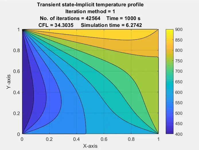
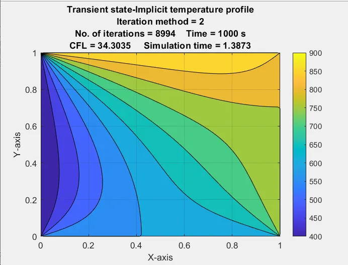
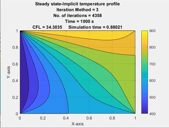
Observation: Iteration time required for Jacobi>Gauss-seidel>Successive over-relaxation

Inference

Number of Iterations for Jacobi>Gauss-seidel>Successive over-relaxation

Steady state method converges faster than transient state.

Since the equations of points are uncoupled in each timestep for explicit method they gives accurate results faster compared to implicit method.