Finding Global Maxima using Genetic Algorithm in Matlab

Introduction

This project is aiming to find the global maxima of a stalagmite function. This can be done by optimizing the input variables to get the peak of the function.

A computer uses algorithms to find solutions to mathematical problems.

Generally there are two kinds of algorithms used to find the solution for optimisation problems.

a) Deterministic algorithm is an algorithm which, given a particular input, will always produce the same output, with the underlying machine always passing through the same sequence of states.Optimization problems usually take so long to get solved using deterministic algorithms so we had to consider stochastic algorithms.

b)Stochastic algorithm refers to a field of optimization algorithms that explicitly use randomness to find the optima of an objective function, or optimize an objective function that itself has randomness (statistical noise)

Genetic Algorithm (ga)

It is a stochastic algorithm technique based on the principles of Genetics and Natural Selection for a search-based optimization. It is frequently used to find optimal or near-optimal solutions to difficult problems which otherwise would take a lifetime to solve.

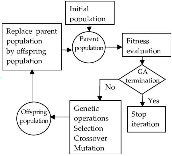
A general description of genetic algorithm:

+ Genetic algorithm starts with an initial set of random solutions called population.

+ Each individual in the population is called a chromosome representing a solution to the problem at hand.

+ The chromosomes evolve through successive iterations, called generations.

+ During each generation, the chromosomes are evaluated using some measures of fitness.

+ To create the next generation, new chromosome, called offspring, are formed by either (a) merging two chromosomes from current generation using a crossover operator or (b) modifying a chromosome using a mutation operator.

+ A new generation is formed by (a) selecting, according to the fitness values, some of the parents and offspring and (b) rejecting others so as to keep the population size constant.

+ Fitter chromosomes have higher probabilities of being selected.

+ After several generations, the algorithms converge to the best chromosome, which hopefully represents the optimum or suboptimal solution to the problem”.

PROGRAM

Using genetic algorithm in matlab we are developing a program to find the global maxima of a stalagmite function.

• Generating stalagmite function

function [F]= stalagmite(input_vector)%'stalagmite is our function template'

x=input_vector(1);
y=input_vector(2);
f1_x=(sin(5.1.*pi.*x+0.5)).^6;
f1_y=(sin(5.1.*pi.*y+0.5)).^6;
f2_x=exp(-4.*log(2).*(x-0.0667).^2./0.64);
f2_y=exp(-4.*log(2).*(y-0.0667).^2./0.64);
F=-(f1_x.*f1_y.*f2_x.*f2_y);

end

• Plotting stalagmite function

clear all
close all
clc
%Defining our search space
x=linspace(0,0.6,150);
y=linspace(0,0.6,150);
% Creating a 2D mesh
[xx yy]=meshgrid(x ,y);
%Evaluating stalagmite function
for i = 1:length(xx)
    for j= 1:length(yy)
        input_vector(1)=xx(i,j);   %2 dimensional array of x values are created
        input_vector(2)=yy(i,j);   %2 dimensional array of y values are created
        f(i,j)=stalagmite(input_vector); %stalagmite function is applied for each x,y 
                                         %coordinates inputs and output values are 
                                         assigned to f(x coordinates(i),y coordinates(j))
        
    end
end

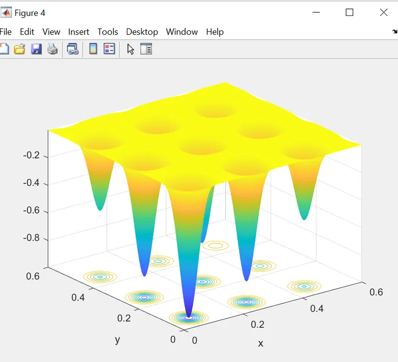
surfc(xx ,yy,f)  %to plot 3D surface of stalagmite function 
xlabel('x')
ylabel('y') 
shading interp   %to give shading interpretation

Stalagamite function

Study 1- Statistical behaviour (unbounded)

%study 1- Statistical behaviour
num_cases=50;% setting number of iterations
tic
for i=1:num_cases;
    [inputs,fopt(i)]= ga (@stalagmite,2);% fopt(fval) is the value of the fitness function at inputs.
                                         %'stalagmite' is the function, 
                                         %2 is number of variables
    xopt(i)=inputs(1);  %storing x values to 'xopt'
    yopt(i)=inputs(2);  %storing y values to 'yopt'
end
study_1_time=toc

figure (1)
%Subplot 1
subplot(2,1,1) %to create a sub plot of 2 row & single column and to select first among that.
surfc(x,y,-f) %surface plotting of stalagmite function
shading interp %shading
hold on        %holding the above plot along the second sub plot
% 'plot3' To plot a set of coordinates connected by line segments, 
plot3(xopt,yopt,-fopt,'marker','o','markersize',5,'markerfacecolor','r')
title('unbounded inputs')

%Subplot 2
subplot(2, 1, 2)%to create a sub plot of 2 row & single column and to select second among that.
plot(-fopt) %to plot the optimum function values (fvals) generated by the genetic algorithm.
xlabel('iterations')
ylabel('function minimum')

Result of study 1

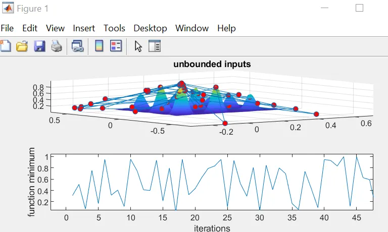
For each iteration optimum value ranges from 0.1 to 1.0.

Study 2- Statistical behaviour(bounded)

Boundary conditions given as [0;0],[0.2;0.2]

%Study 2- Statistical behaviour(bounded)
num_cases=50;% setting number of iterations
tic  %command use to initiate a timer to know calculation time
for i=1:num_cases;
    %Boundary conditions are given to refine the search area '[0;0],[0.6;0.6]' for the global maxima
    [inputs, fopt(i)]= ga(@stalagmite, 2,[],[],[],[],[0;0],[0.6;0.6]);% fopt(fval) is the value of the fitness function at inputs.
                                         %'stalagmite' is the function, 
                                         %2 is number of variables
    xopt(i)=inputs(1)  %storing x values to 'xopt'
    yopt(i)=inputs(2)  %storing y values to 'yopt'
end
study_2_time =toc 
figure (2)

%Subplot 1
subplot(2,1,1) %to create a sub plot of 2 row & single column and to select first among that.
surfc(x,y,-f) %surface plotting of stalagmite function
shading interp %shading
hold on        %holding the above plot along the second sub plot
% 'plot3' To plot a set of coordinates connected by line segments, 
plot3(xopt,yopt,-fopt,'marker','o','markersize',5,'markerfacecolor','r')
title('bounded inputs')

%Subplot 2
subplot(2, 1, 2)%to create a sub plot of 2 row & single column and to select second among that.
plot(-fopt) %to plot the optimum function values (fvals) generated by the genetic algorithm.
xlabel('iterations')
ylabel('function minimum')

Result of study 2

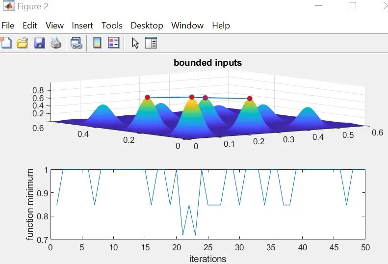
For each iteration value ranges from 0.7 to 1.0

Study 3- Statistical behaviour(giving boundary condition and population size)

Boundary conditions given as [0;0],[0.2;0.2] and initial population size as 400.

%study 3- Statistical behaviour(bounded and population size increased)
num_cases=50;% setting number of iterations
options=optimoptions('ga','PopulationSize',400);
%optimoptions returns options for the 'ga' solver with the named parameters ('PopulationSize') altered with the specified values.

tic
for i=1:num_cases;
   [input,fopt(i)]=ga(@stalagmite,2,[],[],[],[],[0;0],[0.2;0.2],[],[],options);
   % fopt(fval) is the value of the fitness function at inputs.
   %'stalagmite' is the function,'2' is number of variables
   %'options' are used to give initial population size.
    xopt(i)=inputs(1)  %storing x values to 'xopt'
    yopt(i)=inputs(2)  %storing y values to 'yopt
end
study_3_time =toc
figure (3)

%Subplot 1
subplot(2,1,1) %to create a sub plot of 2 row & single column and to select first among that.
surfc(x,y,-f) %surface plotting of stalagmite function
shading interp %shading
hold on        %holding the above plot along the second sub plot
% 'plot3' To plot a set of coordinates connected by line segments, 
plot3(xopt,yopt,-fopt,'marker','o','markersize',5,'markerfacecolor','r')
title('bounded inputs & customized initial population')

%Subplot 2
subplot(2, 1, 2)%to create a sub plot of 2 rows & single column and to select second among that.
plot(-fopt) %to plot the optimum function values (fvals) generated by the genetic algorithm.
xlabel('iterations')
ylabel('function minimum')

Result of study 3

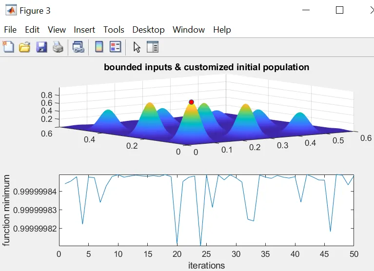
>>xopt3 =0.0668,yopt3 = 0.0668 ,fopt=0.9999998.

Optimum value range is narrowed down to 0.99999981 - 0.99999984. The iteration values have a precision upto 6th decimal place.

Which means more accurate value.

Optimum input value for the maximum function value is xopt3 =0.0668,yopt3 = 0.0668.

Combined program

Program containing all three studies.

clear all
close all
clc
%Defining our search space
x=linspace(0,0.6,150);
y=linspace(0,0.6,150);
% Creating a 2D mesh
[xx yy]=meshgrid(x ,y);
%Evaluating stalagmite function
for i = 1:length(xx)
    for j= 1:length(yy)
        input_vector(1)=xx(i,j);
        input_vector(2)=yy(i,j);
        f(i,j)=stalagmite(input_vector);
        
    end
end
figure(4)
surfc(x ,y,f)
xlabel('x')
ylabel('y')



%study 1- Statistical behaviour
num_cases=50;% setting number of iterations
tic
for i=1:num_cases;
    [inputs,fopt1(i)]= ga (@stalagmite,2);% fopt(fval) is the value of the fitness function at inputs.
                                         %'stalagmite' is the function, 
                                         %2 is number of variables
    xopt1(i)=inputs(1)  %storing x values to 'xopt'
    yopt1(i)=inputs(2)  %storing y values to 'yopt'
end
study_1_time =toc 
figure (1)

%Subplot 1
subplot(2,1,1) %to create a sub plot of 2 rows & single column and to select first among that.
surfc(x,y,-f) %surface plotting of stalagmite function
shading interp %shading
hold on        %holding the above plot along the second sub plot
% 'plot3' To plot a set of coordinates connected by line segments, 
plot3(xopt1,yopt1,-fopt1,'marker','o','markersize',5,'markerfacecolor','r')
title('unbounded inputs')

%Subplot 2
subplot(2, 1, 2)%to create a sub plot of 2 rows & single column and to select second among that.
plot(-fopt1) %to plot the optimum function values (fvals) generated by the genetic algorithm.
xlabel('iterations')
ylabel('function minimum')

%Study 2- Statistical behaviour(bounded)
num_cases=50;% setting number of iterations
tic  %command use to initiate a timer to know calculation time
for i=1:num_cases;
    %Boundary conditions are given to refine the search area '[0;0],[0.6;0.6]' for the global maxima
    [inputs, fopt2(i)]= ga(@stalagmite, 2,[],[],[],[],[0;0],[0.6;0.6]);% fopt(fval) is the value of the fitness function at inputs.
                                         %'stalagmite' is the function, 
                                         %2 is number of variables
    xopt2(i)=inputs(1)  %storing x values to 'xopt'
    yopt2(i)=inputs(2)  %storing y values to 'yopt'
end
study_2_time =toc 
figure (2)

%Subplot 1
subplot(2,1,1) %to create a sub plot of 2 row & single column and to select first among that.
surfc(x,y,-f) %surface plotting of stalagmite function
shading interp %shading
hold on        %holding the above plot along the second sub plot
% 'plot3' To plot a set of coordinates connected by line segments, 
plot3(xopt2,yopt2,-fopt2,'marker','o','markersize',5,'markerfacecolor','r')
title('bounded inputs')

%Subplot 2
subplot(2, 1, 2)%to create a sub plot of 2 row & single column and to select second among that.
plot(-fopt2) %to plot the optimum function values (fvals) generated by the genetic algorithm.
xlabel('iterations')
ylabel('function minimum')


%study 3- Statistical behaviour(bounded and population size increased)
num_cases=50;% setting number of iterations
options=optimoptions('ga','PopulationSize',400);
%optimoptions returns options for the 'ga' solver with the named parameters ('PopulationSize') altered with the specified values.

tic
for i=1:num_cases;
   [input,fopt3(i)]=ga(@stalagmite,2,[],[],[],[],[0;0],[0.2;0.2],[],[],options);
   % fopt(fval) is the value of the fitness function at inputs.
   %'stalagmite' is the function,'2' is number of variables
   %'options' are used to give initial population size.
    xopt3(i)=inputs(1)  %storing x values to 'xopt'
    yopt3(i)=inputs(2)  %storing y values to 'yopt
end
study_3_time =toc
figure (3)
%Subplot 1
subplot(2,1,1) %to create a sub plot of 2 rows & single column and to select first among that.
surfc(x,y,-f) %surface plotting of stalagmite function
shading interp %shading
hold on        %holding the above plot along the second sub plot
% 'plot3' To plot a set of coordinates connected by line segments, 
plot3(xopt3,yopt3,-fopt3,'marker','o','markersize',5,'markerfacecolor','r')
title('bounded inputs & customized initial population')

%Subplot 2
subplot(2, 1, 2)%to create a sub plot of 2 row & single column and to select second among that.
plot(-fopt3) %to plot the optimum function values (fvals) generated by the genetic algorithm.
xlabel('iterations')
ylabel('function minimum')

Result analysis and Conclusion

Study 1 time=2.3791

Study 2 time=2.7139

Study 3 time=13.2147

Maximum function values from study 1= 0.1 to 1.0

Maximum function values from study 2= 0.7 to 1.0

Maximum function values from study 3= 0.99999981 - 0.99999984

Inference

Calculation time increases as the initial population size is increased.

Narrowing the search area by giving boundary conditions for input makes a great difference from study 1 to study 2. Which means for a larger search area genetic algorithm is inapplicable.

In the third study we have increased the population size and also reduced search area. Altogether we could achieve precision upto 6th decimal place. But the change in population size resulted in longer calculation time.

From study 3 we can conclude that,

The maximum function value as 0.9999998 and optimum input value as xopt3 =0.0668,yopt3 = 0.0668.

Error happened while writing program

1: Plotted function values (optimum function values) and stalagmite function surface became unaligned.

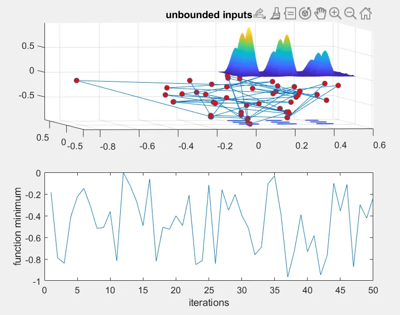
Solution: The stalagmite function is also inverted along inverting the 'plot3' function values. No error messages were given since there were no technical errors.

2:Used colon instead of semicolon while giving boundary conditions.

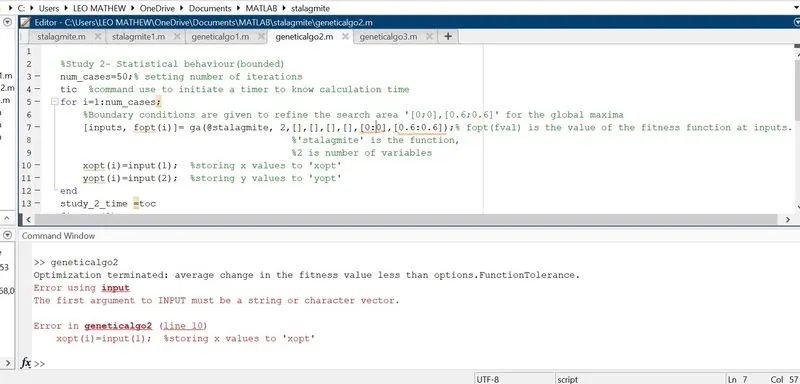
Solution:The problem was a syntax error where the vector dimensions of bounded conditions do not match with our calculation , it is resolved while using semicolon.