Week 3 - Solving second order ODEs

• Aim

• Theory and governing equation

• Developing a program for simulating a simple pendulum

1. Creating an ordinary differential equation function (template function)

2. Solving an ordinary differential equation

3. Creating animation for pendulum motion

• Final program

• Results

Youtube link of the animation

• Error faced while programming

• Aim

To simulate the motion of a simple pendulum and to animate it. A Matlab program can be used to simulate the pendulum motion.The motion is simulated for 20 sec, with an initial angular displacement 0 rad and initial angular velocity 3 rad/sec at time t=0.

• Governing equation

The governing equation for the motion of a simple pendulum is an ODE. The motion of a simple pendulum is angular and it is time dependent.

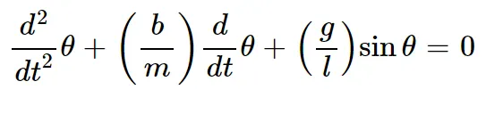
In the above equation,

g = gravity in m/s2,

L = length of the pendulum in m,

m = mass of the ball in kg,

b=damping coefficient.

• Developing a program for simulating a simple pendulum

First we have to solve the ordinary differential equation (ODE) and need to get the results in an array. Then we can simulate the pendulum as an animation.

1.Creating an ordinary differential equation function (template function)

The program below defines the ordinary differential equation. Here we are converting the second order ODE depicting angular velocity to a First order ODE.

Code,

function[dtheta_dt]=ode_func(t,theta,b,g,l,m)
theta1=theta(1)
theta2=theta(2)
dtheta1_dt=theta2;
dtheta2_dt=-(b/m)*theta2-(g/l)*sin(theta1);
dtheta_dt=[dtheta1_dt;dtheta2_dt];
end

• theta1 refers to angular position
• theta2 =dtheta1_dt refers to angular displacement and
• dtheta2_dt refers to angular velocity.
• dtheta2_dt=-(b/m)*theta2-(g/l)*sin(theta1); is our function definition.

This program should be saved in the same name of the template function that is ‘ode_func’.

2.Solving an ordinary differential equation

Code,

clc
b=0.05;
g=9.81;
l=1;
m=0.1;
%initial condition
theta_0=[0;5];
%time points
t_span=linspace(0,10,500);
%solve ODE
[t,results]=ode45(@(t,theta)ode_func(t,theta,b,g,l,m),t_span,theta_0);
%plotting the graph
plot(t,results(:,1))%plotting first column array of results
hold on
plot(t,results(:,2))%plotting second column array of results
ylabel('plot')
xlabel('time')

• [t,results] is the output array ,ode45 is an inbuilt anonymous function
• for solving ordinary differential equations
• t is the independent variable of the ODE ,here in this case it is time.
• theta is the dependent variable 'ode_func()' is the template used to call the function.
• 't,theta,b,g,l,m' are input .
• Here 't_span' and 'theta_0' are considered as the limit for integration and initial condition respectively.

About the anonymous function ‘ode45’.

Ode45 is a function in matlab that solves ordinary or partial differential equations using a numerical method. The numerical method in question here is the 4th order Runge Kutta method.

This doesn't define the ODE. It is an ODE solver program using the Runge Kutta method.

Result

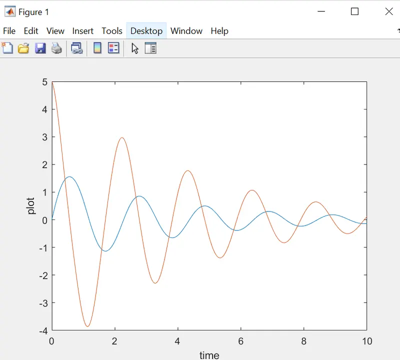
The graph is plotted for both displacement and velocity variation with respect to time.

Red line - velocity curve

Blue line - displacement curve

3.Creating animation for pendulum motion

Here we are plotting a pendulum using plot command. The idea is to plot a line with one end fixed and the coordinates of the other end varying according to the theta values obtained by solving ODE.

Code,

theta=results(:,1); %results are called upon a column array named as theta.

ct=1; % activating counter

for i=1:length(theta);

Theta=theta(i);

l=-1;

%defining coordinates

x0=0;

y0=0;

x1=l*sin(Theta);

y1=l*cos(Theta);

%plotting

plot([x0 x1],[y0 y1],'linewidth',3);

hold on %used to plot bob along the pendulum in each figure.

plot(x1,y1,'o','marker','o','markersize',5,'markerfacecolor','r');%marker in 'o' shape is used to create a bob.

hold off

axis([-1 1 -1 1]); %setting up axis of the figure

pause(0.03); %pause after each result

M(ct)=getframe(gcf); %figures (gcf) are captured using get frame command into the variable M.

ct=ct+1; % defining counter

end

movie(M) %creating movie of contents in M

videofile=VideoWriter('forward_kinematics.avi','Uncompressed AVI');% video file is made by video writer

open(videofile)

writeVideo(videofile,M)% writing the created movie M to the video file.

close(videofile)

• Final program

clear all
close all
clc
  b=0.05;
  g=9.81;
  l=1;
  m=1;
%initial condiition
  theta_0=[0;3];
%time points
  t_span=linspace(0,20,500);
%solve ODE
  [t,results]=ode45(@(t,theta)ode_func(t,theta,b,g,l,m),t_span,theta_0);
%[t,results] is the output array ,ode45 is an in buit anonymous function
%for solving ordinary differential equations
%t is the independent variable of the ODE ,here in this case it is time.
%theta is the dependent variable 'ode_func()' is the template used to call
%the function.'t,theta,b,g,l,m' are input values.Here 't_span' and 'theta_0' are considered as the limit for
%integration and initial condition
  theta=results(:,1);
  ct=1;
for i=1:length(theta);
    Theta=theta(i);
  l=-1;
  x0=0;
  y0=0;
  x1=l*sin(Theta);
  y1=l*cos(Theta);
  %plotting
  plot([x0 x1],[y0 y1],'linewidth',3);
 hold on
  plot(x1,y1,'o','marker','o','markersize',5,'markerfacecolor','r');
  %marker in 'o' shape is used to create a bob.
 hold off
  title('pendulum')
  axis([-1 1  -1 1]);
  pause(0.03);
  M(ct)=getframe(gcf);
%figures (gcf) are captured ufsing get frame command into the variable M. 
  ct=ct+1;
end    
movie(M) % movie is formed using contents in M.
videofile=VideoWriter('forward_kinematics.avi','Uncompressed AVI');% video file is made by video writer
open(videofile)
writeVideo(videofile,M) % writing the created movie M to the video file.
close(videofile)

• Result

Youtube link of the animation :https://youtu.be/bgiwHOCjCPQ

• Error faced while programming

1.Failed to use hold off command

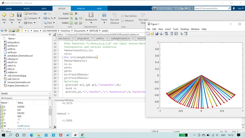
Solution: Use hold off command after the plot command for pendulum bob.

2.Pendulum swings invertedly

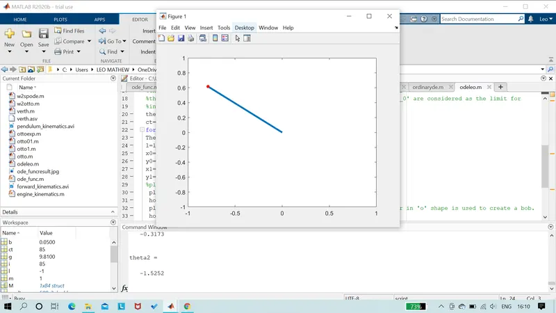
Solution: Give length of the pendulum as negative(-l).