Week 3.5 - Deriving 4th order approximation of a 2nd order derivative using Taylor Table method
Deriving 4th order approximation of a 2nd order derivative using Taylor Table method
Content
- Derivation of 4th order approximations of the second-order derivative.
- Matlab code to compare all three errors based on variation in dx
- Result and inferance
- Question; describe why a skewed scheme is useful? What can a skewed scheme do that a CD scheme cannot?
Derivation of 4th order approximations of the second-order derivative.
- By Central difference Method
The order of accuracy P = Number of nodes in the stencil N - order of derivative Q + 1 for symmetric/central schemes
Here we want order of accuracy four and order of derivative two, so number of nodes in our stencil is five.
*...............*...............*...............*...............*
i-2 i-1 0 i+1 i+2
`af(i-2)=af(i)-af'(i)2Deltax+(af''(i)(2Deltax)^2)/(2!)-(af'''(i)(2Deltax)^3)/(3!)+(af''''(i)(2Deltax)^4)/(4!)-(af'''''(i)(2Deltax)^5)/(5!)+...`
`bf(i-1)=bf(i)-bf'(i)Deltax+(bf''(i)(Deltax)^2)/(2!)-(bf'''(i)(Deltax)^3)/(3!)+(bf''''(i)(Deltax)^4)/(4!)-(bf'''''(i)(Deltax)^5)/(5!)+...`
`cf(i)=cf(i)`
`df(i+1)=df(i)+df'(i)Deltax+(df''(i)(Deltax)^2)/(2!)+(df'''(i)(Deltax)^3)/(3!)+(df''''(i)(Deltax)^4)/(4!)+(df'''''(i)(Deltax)^5)/(5!)+...`
`ef(i+2)=af(i)+af'(i)2Deltax+(af''(i)(2Deltax)^2)/(2!)+(af'''(i)(2Deltax)^3)/(3!)+(af''''(i)(2Deltax)^4)/(4!)+(af'''''(i)(2Deltax)^5)/(5!)+...`
By arranging the above taylor series expansions in a table we get the taylor table shown below,
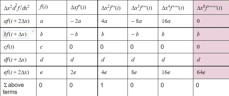
The fourth order approximation equation for `(d^2u)/dx^2` is;
`(d^2u)/dx^2`= `(af(i)+bf(i+1)+cf(i+2)+df(i+3)+ef(i+4)+gf(i+5))/(Deltax)^2`..................................(a)
Now from our taylor table `(d^2u)/dx^2`=
`(a+b+c+d+e+g)f(i)+(-2a-b+0+d+2e)f’’(i)Deltax+(4a+b+0+d+4e)f’’(i)Deltax^2)/(2!)+(-8a-b+0-+d+8e)f’''(i)Deltax^3)/(3!)+(16a+b+0+d+16e)f’''(i)Deltax^4)/(4!)+(64a+b+0+d+64e)f’''(i)Deltax^6)/(6!)`
……………………………….(1)
The coefficients of terms `f(i)` `Deltaxf'(i)/1!``Deltax3f'''(i)/3!``Deltax4f''''(i)/5!``Deltax5f'''''(i)/5!` `Deltax6f''''''(i)/6!` are zero.
`Deltax2f''(i)/2!` =1
Dividing through out by`Deltax^2`
Now from our taylor table `(d^2u)/dx^2`=
`(0+0.5b+2c+4.5d+8e+12.5g)f’’(i)+1.0125d+5.688e+21.701g)f’’’’’’(i)Deltax^4``
Here in the above equation we can see the truncation error is of order four.
Solving the above equations using matrix inverse method we can get the coefficient values as;
a=-5/60
b=4/3
c=-5/2
d=4/3
e=-5/60
Final centered fourth order equation for second order derivative by substituting coefficients in equation (a) we get;
`(d^2u)/dx^2`=`((-5/60)f(i)+(4/3)f(i-1)+(-5/2)f(i-2)+-13f(i-3)+(4/3)f(i-4)+(-5/60)f(i-5))/(Deltax)^2`
Error in central skewed method = above centre skewed equation - analytical solution.
Now we have to compare the above error with the other two errors for the variation in dx.
- By Right-Sided Skewed Method
The order of accuracy P = Number of nodes in the stencil N - order of derivative Q for one-sided/skewed schemes
Here we want order of accuracy four and order of derivative two, so number of nodes in our stencil is six.
*...............*...............*...............*...............*...............*
i i+1 i+2 i+3 i+4 i+5
`af(i)=af(i)`
`bf(i+1)=bf(i)+bf'(i)Deltax+(bf''(i)(Deltax)^2)/(2!)+(bf'''(i)(Deltax)^3)/(3!)+(bf''''(i)(Deltax)^4)/(4!)+(bf'''''(i)(Deltax)^5)/(5!)+...`
`cf(i+2)=cf(i)+cf'(i)2Deltax+(cf''(i)(2Deltax)^2)/(2!)+(cf'''(i)(2Deltax)^3)/(3!)+(cf''''(i)(2Deltax)^4)/(4!)+(cf'''''(i)(2Deltax)^5)/(5!)+...`
`df(i+3)=df(i)+df'(i)Deltax+(df''(i)(3Deltax)^2)/(2!)+(df'''(i)(3Deltax)^3)/(3!)+(df''''(i)(3Deltax)^4)/(4!)+(df'''''(i)(3Deltax)^5)/(5!)+...`
`ef(i+4)=af(i)+af'(i)4Deltax+(af''(i)(2Deltax)^2)/(2!)+(af'''(i)(2Deltax)^3)/(3!)+(af''''(i)(2Deltax)^4)/(4!)+(af'''''(i)(2Deltax)^5)/(5!)+...`
`gf(i+5)=gf(i)+gf'(i)5Deltax+(gf''(i)(5Deltax)^2)/(2!)+(gf'''(i)(5Deltax)^3)/(3!)+(gf''''(i)(5Deltax)^4)/(4!)+(gf'''''(i)(5Deltax)^5)/(5!)+...`
By arranging the above taylor series expansions in a table we get the taylor table shown below,
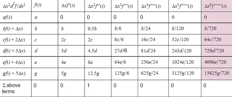
The fourth order approximation equation for `(d^2u)/dx^2` is;
`(d^2u)/dx^2`=`(af(i)+bf(i+1)+cf(i+2)+df(i+3)+ef(i+4)+gf(i+5))/(Deltax)^2`..................................(b)
Now from our taylor table `(d^2u)/dx^2`=
`(a+b+c+d+e+g)f(i)+(0+b+2c+3d+4e+5g)f’(i)Deltax+(0+0.5b+2c+4.5d+8e+12.5g)f’’(i)Deltax^2+(0+b/6+1.333c+4.5d+10.666e+20.833g)f’’’(i)Deltax^3+(0+b/24+.666c+3.375d+10.666e+26.041g)f’’’’(i)Deltax^4+(0+b/120+.266c+2.025d+8.533e+26.041g)f’’’’’(i)Deltax^5+(0+b/720+.088c+1.0125d+5.688e+21.701g)f’’’’’’(i)Deltax^6`……………………………….(2)
The coefficients of terms `f(i)` `Deltaxf'(i)/1!``Deltax3f'''(i)/3!``Deltax4f''''(i)/5!``Deltax5f'''''(i)/5!` `Deltax6f''''''(i)/6!` are zero.
`Deltax2f''(i)/2!` =1
Dividing through out by`Deltax^2`
Now from our taylor table `(d^2u)/dx^2`=
`(0+0.5b+2c+4.5d+8e+12.5g)f’’(i)+1.0125d+5.688e+21.701g)f’’’’’’(i)Deltax^4``
Here in the above equation we can see the truncation error is of order four.
(a+b+c+d+e+g)=0,
(0+b+2c+3d+4e+5g)=0,
(0+0.5b+2c+4.5d+8e+12.5g)=1,
(0+b/6+1.333c+4.5d+10.666e+20.833g)=0,
(0+b/24+.666c+3.375d+10.666e+26.041g)=0,
(0+b/120+.266c+2.025d+8.533e+26.041g)=0,
(0+b/720+.088c+1.0125d+5.688e+21.701g)=0
Solving the above equations using matrix inverse method we can get the coefficient values as;
a=3.75;
b=-77/6;
c=107/6;
d=-13;
e=61/12;
g=-5/6;
Final right sided fourth order equation for second order derivative by substituting coefficients in equation (b) we get;
`(d^2u)/dx^2`=`(3.75f(i)+(-77/6)f(i-1)+(107/6)f(i-2)+-13f(i-3)+(61/12)f(i-4)+(-5/6)f(i-5))/(Deltax)^2`
Error in left skewed method = above right sided equation - analytical solution.
Now we have to compare the above error with the other two errors for the variation in dx.
- By left-Sided Skewed Method
The order of accuracy P = Number of nodes in the stencil N - order of derivative Q for one-sided/skewed schemes
Here we want order of accuracy four and order of derivative two, so the number of nodes in our stencil is six.
*...............*...............*...............*...............*...............*
i-5 i-4 i-3 i-2 i-1 i
`af(i)=af(i)`
`bf(i-1)=bf(i)-bf'(i)Deltax+(bf''(i)(Deltax)^2)/(2!)-(bf'''(i)(Deltax)^3)/(3!)+(bf''''(i)(Deltax)^4)/(4!)-(bf'''''(i)(Deltax)^5)/(5!)+...`
`cf(i-2)=cf(i)-cf'(i)2Deltax+(cf''(i)(2Deltax)^2)/(2!)-(cf'''(i)(2Deltax)^3)/(3!)+(cf''''(i)(2Deltax)^4)/(4!)-(cf'''''(i)(2Deltax)^5)/(5!)+...`
`df(i-3)=df(i)-df'(i)Deltax+(df''(i)(3Deltax)^2)/(2!)-(df'''(i)(3Deltax)^3)/(3!)+(df''''(i)(3Deltax)^4)/(4!)-(df'''''(i)(3Deltax)^5)/(5!)+...`
`ef(i-4)=af(i)-af'(i)4Deltax+(af''(i)(2Deltax)^2)/(2!)-(af'''(i)(2Deltax)^3)/(3!)+(af''''(i)(2Deltax)^4)/(4!)-(af'''''(i)(2Deltax)^5)/(5!)+...`
`gf(i-5)=gf(i)-gf'(i)5Deltax+(gf''(i)(5Deltax)^2)/(2!)-(gf'''(i)(5Deltax)^3)/(3!)+(gf''''(i)(5Deltax)^4)/(4!)(gf'''''(i)(5Deltax)^5)/(5!)+...`
By arranging the above taylor series expansions in a table we get the taylor table shown below,
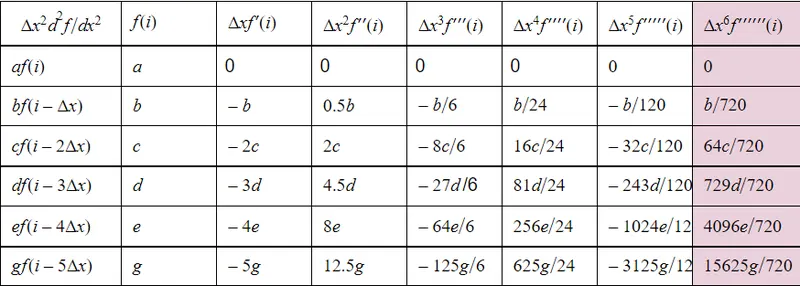
The fourth order approximation equation for `(d^2u)/dx^2` is;
`(d^2u)/dx^2`= `(af(i)+bf(i-1)+cf(i-2)+df(i-3)+ef(i-4)+gf(i-5))/(Deltax)^2`..........................................(c)
Now from our taylor table `(d^2u)/dx^2`=
`(a+b+c+d+e+g)f(i)+(0-b-2c-3d-4e-5g)f’(i)Deltax+(0+0.5b+2c+4.5d+8e+12.5g)f’’(i)Deltax^2+(0-b/6-1.333c-4.5d-10.666e-20.833g)f’’’(i)Deltax^3+(0+b/24+.666c+3.375d+10.666e+26.041g)f’’’’(i)Deltax^4+(0-b/120-.266c-2.025d-8.533e-26.041g)f’’’’’(i)Deltax^5+(0+b/720+.088c+1.0125d+5.688e+21.701g)f’’’’’’(i)Deltax^6` ……………………………….(3)
The coefficients of terms `f(i)` `Deltaxf'(i)/1!``Deltax3f'''(i)/3!``Deltax4f''''(i)/5!``Deltax5f'''''(i)/5!` `Deltax6f''''''(i)/6!` are zero.
`Deltax2f''(i)/2!` =1
Dividing through out by`Deltax^2`
Now from our taylor table `(d^2u)/dx^2`=
`(0+0.5b+2c+4.5d+8e+12.5g)f’’(i)+1.0125d+5.688e+21.701g)f’’’’’’(i)Deltax^4``
Here in the above equation we can see the truncation error is of order four.
(a+b+c+d+e+g)=0,
(0-b-2c-3d-4e-5g)=0,
(0+0.5b+2c+4.5d+8e+12.5g)=1,
(0-b/6-1.333c-4.5d-10.666e-20.833g)=0,
(0+b/24+.666c+3.375d+10.666e+26.041g)=0,
(0-b/120-.266c-2.025d-8.533e-26.041g)=0,
(0+b/720+.088c+1.0125d+5.688e+21.701g)=0
Solving the above equations using matrix inverse method we can get the coefficient values as;
a=3.75;
b=-77/6;
c=107/6;
d=-13;
e=61/12;
g=-5/6;
Final left sided fourth order equation for second order derivative by substituting coefficients in equation (c) we get;
`(d^2u)/dx^2`= `(3.75f(i)+(-77/6)f(i-1)+(107/6)f(i-2)+-13f(i-3)+(61/12)f(i-4)+(-5/6)f(i-5))/(Deltax)^2`
Error in left skewed method = above left sided equation - analytical solution.
Compare the above error with other two errors for the variation in dx.
Matlab code to compare all three errors based on variation in dx
Main Code
clear all
close all
clc
x=pi/3;%Value of x
dx=linspace(pi/4,pi/400,40);%Range of dx(gradient of differential)
for i=1:length(dx)% Using for loop algorithm
    error_fourthorder_centre(i)=fourthorder_centreskew_sndderivative(x,dx(i));
    error_fourthorder_right(i)=fourthorder_rightskew_sndderivative(x,dx(i));
    error_fourthorder_left(i)=fourthorder_leftskew_sndderivative(x,dx(i));
end
figure(1)% calling the figure function of Matlab.
%plotting the log graph of the function to see the function as a straight line and to see plot for a large range
loglog(dx,error_fourthorder_centre,'r','marker','*')
hold on % to include other plots in same fig.
loglog(dx,error_fourthorder_right,'g','marker','o')
loglog(dx,error_fourthorder_left,'b','marker','diamond')
xlabel('\leftarrow  dx')
ylabel('Error')
hold off
legend('error_fourthorder_centre','error_fourthorder_right','error_fourthorder_left')%to distinguish between plots
Function code symmetric/centered
function out=fourthorder_centreskew_sndderivative(x,dx)


%analytical function =exp(x)*cos(x);
%Analytical %Second derivative
analytical_derivative =-2*exp(x)*sin(x);
%Numerical Second derivative
p=x-2*dx;
q=x-dx;
r=x+dx;
s=x+2*dx;
a=-5/60
b=4/3
c=-5/2
d=4/3
e=-5/60
%fourthorder_centreskew_sndderivative=(a*f(x-2*dx)+b*f(x-dx)+c*f(x)+d*f(x+dx)+e*f(x+2*dx))/(dx^2);
%
centreskew_difference=(a*exp(p)*cos(p)+b*exp(q)*cos(q)+c*exp(x)*cos(x)+d*exp(r)*cos(r)+e*exp(s)*cos(s))/(dx^2);
out=abs(centreskew_difference-analytical_derivative);
end
Function code right sided
function out=fourthorder_rightskew_sndderivative(x,dx)


%analytical function =exp(x)*cos(x);

%Analytical second order derivative

analytical_derivative =-2*exp(x)*sin(x);

%Numerical second order derivative


%fourthorder_rightskew_sndderivative=(a*f(x)+b*f(x+dx)+c*f(x+2*dx)+d*f(x+3*dx)+e*f(x+4*dx)+g*f(x+5*dx))/(12*dx^2);

p=x+dx;
q=x+2*dx;
r=x+3*dx;
s=x+4*dx;
t=x+5*dx;

a=3.75;
b=-77/6;
c=107/6;
d=-13;
e=61/12;
g=-5/6;

rightskew_derivative=(a*exp(x)*cos(x)+b*exp(p)*cos(p)+c*exp(q)*cos(q)+d*exp(r)*cos(r)+e*exp(s)*cos(s)+g*exp(t)*cos(t))/(dx^2);

out=abs(rightskew_derivative-analytical_derivative);

end
Function code left sided
function out=fourthorder_leftskew_sndderivative(x,dx)

%analytical function =exp(x)*cos(x);
%Analytical first derivative
analytical_derivative =-2*exp(x)*sin(x);
%Numerical first derivative

%fourthorder_leftskew_sndderivative=(a*f(x)+b*f(x-dx)+c*f(x-2*dx)+d*f(x-3*dx)+e*f(x-4*dx))+g(x-5*dx)/(12*dx^2);
p=x-dx
q=x-2*dx
r=x-3*dx
s=x-4*dx
t=x-5*dx;
a=3.75;
b=-77/6;
c=107/6;
d=-13;
e=61/12;
g=-5/6;

leftskew_derivative=(a*exp(x)*cos(x)+b*exp(p)*cos(p)+c*exp(q)*cos(q)+d*exp(r)*cos(r)+e*exp(s)*cos(s)+g*exp(t)*cos(t))/(dx^2);
out=abs(leftskew_derivative-analytical_derivative);
end
Result and inferance
Result
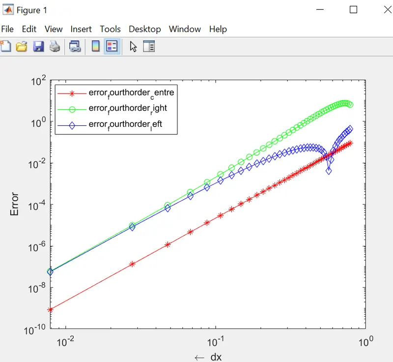
The graphs of centre, right and left skewd error V/S gradient dx were ploted.
Inference
Symmetric method gives us least amount of error compared to skewed methods as gradient is decreased.
The skewed methods can give higher order approximation even by using information from 1 stencil point less than skewed scheme.
Question; describe why a skewed scheme is useful? What can a skewed scheme do that a CD scheme cannot?
Skewed scheme is useful at boundary points where information from both sides are not available. Central differencing or symmetric scheme of finate difference method can't be used at the boundary points, where the information from left and right sides are not available in such cases skewed scheme is the only option..