Week 5.1 - Mid term project - Solving the steady and unsteady 2D heat conduction problem

5.1 - Solving the steady and unsteady 2D heat conduction problem

OBJECTIVE

1. Solve the 2D heat conduction equation by using the point iterative techniques for both steady and transient conditions
2. Write code for both implicit and explicit schemes (Transient analysis only)
3. Compare the convergence rate (Number of iterations) of the steady state and transient [explicit and implicit] simulations and justify the numerics

GIVEN DATA

• The Boundary conditions for the problem are as follows:

  Top Boundary = 600 K

  Bottom Boundary = 900 K

  Left Boundary = 400 K

  Right Boundary = 800 K

• Absolute error criteria = 1e-4

THEORY

• The governing equation for 2D transient state heat conduction without heat generation is,

`(delT)/(delt)=alpha((del^2T)/(delx^2)+(del^2T)/(dely^2))`

• The governing equation for 2D steady-state heat conduction without heat generation is,

`(del^2T)/(delx^2)+(del^2T)/(dely^2) = 0`

DISCRETIZATION

• The central differencing scheme is used to discretize the second-order PDE of T wrt x and y as it is elliptical in nature and takes information from all sides.
• The forward differencing scheme is used to discretize the time derivative term as it is hyperbolic in nature and takes information from left to right.
• At any node (i,j) temperature is represented by T_i,j.
• `{partial ^{2}T}/{partial x^{2}} = (T_{i-1,j} - 2*T_{i,j}+ T_{i+1,j})/(dx^2)`
• `{partial ^{2}T}/{partial y^{2}} = (T_{i,j+1} - 2*T_{i,j}+ T_{i,j-1})/(dy^2)`
• `{partial T}/{partial t} = (T_{i,j}^{n+1} - T_{i,j}^{n})/(dt)`

Steady State Analysis

• The governing equation for 2D steady state can be discretized as

`T_[i,j] = 1/k((T_[i-1,j]+T_[i+1,j])/(dx^2)+(T_[i,j-1]+T_[i,j+1])/(dy^2))`

where `k = 2*(dx^2 + dy^2)/(dx^2 * dy^2)`

• This equation can be solved with the help of iterative solvers like Jacobi, Gauss-Siedel, and Successive Over Relaxation (SOR).

1. Jacobi Method - In this method old value of temperature is used to evaluate the temperature at the next node.
2. Gauss-Seidel Method - This method is similar to the Jacobi method but here the most updated temperature value is used to compute the temperature of the next node.
3. Successive Over Relaxation (SOR) method - This method is an improvisation of the Gauss-Seidel iterative method. Here a relaxing factor (w) is used. If the value of w is less than 1, it is under relaxation. If the value of w is greater than 1, it is over-relaxation.

MATLAB CODE FOR STEADY-STATE ANALYSIS

Main Program

% Solving Steady state 2D heat conduction equation

clear all
close all
clc

% Inputs
nx = 10;  % Number of grid points along the x-axis
ny = nx;   % Number of grid points along the y-axis
L = 1;     % Domain length in x and y direction

x = linspace(0,L,nx);
dx = x(2)-x(1);
y = linspace(0,L,ny);
dy= y(2)-y(1);
[xx,yy] = meshgrid(x,y);

% Initialising arrays and assigning boundary conditions
T = 300*ones(nx,ny);
T(:,1) = 400;  % Left Boundary
T(1,:) = 600;  % Top Boundary
T(end,:) = 900;  % Bottom Boundary
T(:,end) = 800;  % Right Boundary

% Temperature values at corner nodes
T(1,1) = 500;
T(1,end) = 700;
T(end,1) = 650;
T(end,end) = 850;

error = 9e9; % Assumed initial value of error
tol = 1e-4;  % Tolerance value

Told = T;  % Told is the temperature from the previous iteration

k = 2*((1/dx^2)+(1/dy^2));

counter=input('Enter the number for choosing the iterative solver \n Jacobi=1 \n Gauss Seidel=2 \n SOR=3 \n Solver Type: ');

if counter==1  % Jacobi method
    jacobi_solution = jacobi_method(nx,ny,dx,dy,xx,yy,T,Told,error,tol,k);
end
if counter==2   % Gauss Seidel method
        gs_solution = gs_method(nx,ny,dx,dy,xx,yy,T,Told,error,tol,k);
end
if counter==3    % Successive Over Relaxation method
        sor_solution = sor_method(nx,ny,dx,dy,xx,yy,T,Told,error,tol,k);
end

Function for the Jacobi method

% Function to solve using the Jacobi method

function [output] = jacobi_method(nx,ny,dx,dy,xx,yy,T,Told,error,tol,k)

jacobi_iter = 1;
while(tol<error)
    for i = 2:nx-1
        for j =2:ny-1
            Term1 = (Told(i-1,j) + Told(i+1,j))/(k*dx^2);
            Term2 = (Told(i,j+1) + Told(i,j-1))/(k*dy^2);
            T(i,j) = Term1 + Term2;
        end
    end
    error = max(max(abs(Told-T)));
    Told = T;
    jacobi_iter = jacobi_iter + 1;   % To count the number of iterations

    % Plotting the temperature distribution in the domain
    figure(1)
    % plotting contour graph
    [a,b] = contourf(xx,yy,T); 
    % Labelling each curve in the contour graph from the data points of a & b
    clabel(a,b)
    % Indicating chart color pattern
    colormap(jet)
    % Turning on the color bar
    colorbar
    
    % Setting the y-direction axis in reverse order
    set(gca,'ydir','reverse')
    % Inserting title to mention the number of iterations
    title(sprintf('Jacobi Iteration = %d\n Iteration', jacobi_iter))
    % X & Y axis labels
    xlabel('X Axis')
    ylabel('Y Axis')
end
output = jacobi_iter;

Function for the Gauss-Seidel method

% Function to solve using the Gauss-Seidel method

function [output] = gs_method(nx,ny,dx,dy,xx,yy,T,Told,error,tol,k)

gs_iter = 1;
while(tol<error)
    for i = 2:nx-1
        for j =2:ny-1
            Term1 = (T(i-1,j) + Told(i+1,j))/(k*dx^2);
            Term2 = (Told(i,j+1) + T(i,j-1))/(k*dy^2);
            T(i,j) = Term1 + Term2;
        end
    end
    error = max(max(abs(Told-T)));
    Told = T;
    gs_iter = gs_iter + 1;   % To count the number of iterations

    % Plotting the temperature distribution in the domain
    figure(1)
    % plotting contour graph
    [a,b] = contourf(xx,yy,T); 
    % Labelling each curve in the contour graph from the data points of a & b
    clabel(a,b)
    % Indicating chart color pattern
    colormap(jet)
    % Turning on the color bar
    colorbar
    
    % Setting the y-direction axis in reverse order
    set(gca,'ydir','reverse')
    % Inserting title to mention the number of iterations
    title(sprintf('Gauss-Seidel Iteration = %d\n Iteration', gs_iter))
    % X & Y axis labels
    xlabel('X Axis')
    ylabel('Y Axis')
end
output = gs_iter;

Function for the SOR method

% Function to solve using the SOR method

function [output] = sor_method(nx,ny,dx,dy,xx,yy,T,Told,error,tol,k)

omega = 1.2;
sor_iter = 1;
while(tol<error)
    for i = 2:nx-1
        for j =2:ny-1
            Term1 = (T(i-1,j) + Told(i+1,j))/(k*dx^2);
            Term2 = (Told(i,j+1) + T(i,j-1))/(k*dy^2);
            T_gs = Term1 + Term2;
            T(i,j) = (1-omega)*(Told(i,j)) + omega*(T_gs);
        end
    end
    error = max(max(abs(Told-T)));
    Told = T;
    sor_iter = sor_iter + 1;   % To count the number of iterations

    % Plotting the temperature distribution in the domain
    figure(1)
    % plotting contour graph
    [a,b] = contourf(xx,yy,T); 
    % Labelling each curve in the contour graph from the data points of a & b
    clabel(a,b)
    % Indicating chart color pattern
    colormap(jet)
    % Turning on the color bar
    colorbar
    
    % Setting the y-direction axis in reverse order
    set(gca,'ydir','reverse')
    % Inserting title to mention the number of iterations
    title(sprintf('SOR Iteration = %d\n Iteration', sor_iter))
    % X & Y axis labels
    xlabel('X Axis')
    ylabel('Y Axis')
end
output = sor_iter;

Transient State Analysis

• The governing equation for the 2D unsteady state can be discretized as

`frac{T(i,j)^(n+1)-T(i,j)^n}{dt}=alpha**(frac{(Ti,j+1)+(Ti,j-1)-2Ti,j}{dy^2}+frac{(Ti+1,j)+(Ti-1,j)-2Ti,j}{dx^2})`

• This can be further rearranged as,

`T(i,j)^(n+1)=T(i,j)^n+frac{alpha**dt**((Ti,j+1)+(Ti,j-1)-2Ti,j)){dy^2}+frac{alpha**dt**((Ti+1,j)+(Ti-1,j)-2Ti,j)}{dx^2}`

`K1=α(Δt)/(Δx^2)` and `K2=α(Δt)/(Δy^2)`

`T(i,j)^(n+1)**(1+(2**K1)+(2**K2))=T(i,j)^n+K2**((T(i,j+1)^(n+1))+(T(i,j-1)^(n+1))+K1**((T(i+1,j)^(n+1))+(T(i-1,j)^(n+1))`

• The above equation is the explicit equation and it is solved for the nth time step. All the values in the RHS can be calculated easily without the use of iterative solvers since the values are known from the previous iteration.
• The implicit form of the equation is,

`T(i,j)^(n+1)=frac{T(i,j)^n+K2**((T(i,j+1)^(n+1))+(T(i,j-1)^(n+1)))+K1**((T(i+1,j)^(n+1))+(T(i-1,j)^(n+1)))}{1+(2**K1)+(2**K2)}`

In this case, we need to use iterative solvers as temperature values for the next timestep are not known to us.

MATLAB CODE FOR TRANSIENT STATE ANALYSIS (EXPLICIT METHOD)

Main Program

% Solving Transient state 2D heat conduction equation
% Explicit scheme

clear all
close all
clc

% Inputs
nx = 10;  % Number of grid points along the x-axis
ny = nx;   % Number of grid points along the y-axis
L = 1;     % Domain length in x and y direction
alpha = 1.4;  % Diffusivity
dt = 1e-3;

x = linspace(0,L,nx);
dx = x(2)-x(1);
y = linspace(0,L,ny);
dy= y(2)-y(1);
[xx,yy] = meshgrid(x,y);

% Initialising arrays and assigning boundary conditions
T = 300*ones(nx,ny);
T(:,1) = 400;  % Left Boundary
T(1,:) = 600;  % Top Boundary
T(end,:) = 900;  % Bottom Boundary
T(:,end) = 800;  % Right Boundary

% Temperature values at corner nodes
T(1,1) = 500;
T(1,end) = 700;
T(end,1) = 650;
T(end,end) = 850;

error = 9e9; % Assumed initial value of error
tol = 1e-4;  % Tolerance value

Told = T;  % Told is the temperature from the previous iteration

% Calculating CFL numbers
k1 = alpha*(dt/dx^2);
k2 = alpha*(dt/dy^2);
CFL = k1+k2;

iter_counter = 1;
for nt = 1:1400   % Time loop
    for i = 2:nx-1    % Space loop
        for j = 2:ny-1
            Term1 = Told(i-1,j) - 2*T(i,j) + T(i+1,j);
            Term2 = Told(i,j+1) - 2*T(i,j) + T(i,j-1);
            T(i,j) = Told(i,j) + k1*Term1 + k2*Term2;
        end
    end
    Told = T;
    iter_counter = iter_counter +1;

     % Plotting the temperature distribution in the domain
    figure(1)
    % plotting contour graph
    [a,b] = contourf(xx,yy,T); 
    % Labelling each curve in the contour graph from the data points of a & b
    clabel(a,b)
    % Indicating chart color pattern
    colormap(autumn)
    % Turning on the color bar
    colorbar
    
    % Setting the y-direction axis in reverse order
    set(gca,'ydir','reverse')
    % Inserting title to mention the number of iterations
    title(sprintf('Explicit Method \n Number of Iterations = %d Iterations \n CFL Number = %0.4f', iter_counter,CFL))
    % X & Y axis labels
    xlabel('X Axis')
    ylabel('Y Axis')
end

MATLAB CODE FOR TRANSIENT STATE ANALYSIS (IMPLICIT METHOD)

Main Program

% Solving 2D heat conduction equation
% Implicit Scheme
% Transient/Unsteady state condition

clear all
close all
clc

%% Grid points and Inputs
nx = 10;
ny = nx;
L = 1; % length of square domain
nt = 1400; % number of time steps
dt = 0.001; % time step
alpha = 1.4; % diffusivity


%% Creating mesh
x = linspace(0,L,nx); % Number of nodes in X - direction
y = linspace(0,L,ny); % Number of nodes in Y - direction
dx = x(2) - x(1); % step size in x
dy = dx; % step size in y
[xx,yy] = meshgrid(x,y); % mesh grid


%% Calculating Courant numbers (CFL values)
k1 = alpha*(dt/(dx^2));
k2 = alpha*(dt/(dy^2));

%% Boundary Conditions
T = ones(nx,ny);
% inserting temperature values at the corners of the domain
T(:,1) = 400; % Left boundary 
T(1,:) = 600; % Top boundary
T(:,end) = 800; % Right boundary
T(end,:) = 900; % Bottom boundary

%% Calculating 4 corner nodes' temperature values
T(1,1) = (600 + 400)/2;
T(1,end) = (800 + 600)/2;
T(end,1) = (400 + 900)/2;
T(end,end) = (800 + 900)/2;

Tprev = T; % value of previous time step
Told = T; % value of previous iteration

%%  Prompt window

iter_solver = input('Enter the number for choosing the iterative solver \n Jacobi=1 \n Gauss Seidel=2 \n SOR=3 \n Iterative Solver: ');

%%  Iterative Solvers
% Jacobi Iterative method

if iter_solver == 1 
jacobi_iter = 1;
for nt = 1:1400   % Time loop
error = 9e9; % Assumed initial value of error
tol = 1e-4;  % Tolerance value
  while(tol<error)   % Convergence loop
    for i = 2:nx-1     % space loop
        for j =2:ny-1
            Term1 = 1/(1+(2*k1)+(2*k2));
            Term2 = (k1*(Told(i-1,j)+(Told(i+1,j))))+(k2*(Told(i,j-1)+(Told(i,j+1))));
            T(i,j) = Term1*(Tprev(i,j)+Term2);
        end
    end
    error = max(max(abs(Told-T)));
    Told = T;
    jacobi_iter = jacobi_iter + 1;   % To count the number of iterations
  end
 Tprev = T;

 
    % Plotting the temperature distribution in the domain
    figure(1)
    % plotting contour graph
    [a,b] = contourf(xx,yy,T); 
    % Labelling each curve in the contour graph from the data points of a & b
    clabel(a,b)
    % Indicating chart color pattern
    colormap(jet)
    % Turning on the color bar
    colorbar
    
    % Setting the y-direction axis in reverse order
    set(gca,'ydir','reverse')
    % Inserting title to mention the number of iterations
    title(sprintf('Jacobi Iteration (Transient Analysis) = %d Iterations \n Implicit Method', jacobi_iter))
    pause(0.003)
    % X & Y axis labels
    xlabel('X Axis')
    ylabel('Y Axis')
end     
    
% Gauss Seidel Iterative method
elseif iter_solver == 2 
                
gs_iter = 1;
for nt = 1:1400   % Time loop
error = 9e9; % Assumed initial value of error
tol = 1e-4;  % Tolerance value
while(tol<error)   % Convergence loop
    for i = 2:nx-1     % space loop
        for j =2:ny-1
            Term1 = 1/(1+(2*k1)+(2*k2));
            Term2 = (k1*(T(i-1,j)+(T(i+1,j))))+(k2*(T(i,j-1)+(T(i,j+1))));
            T(i,j) = Term1*(Tprev(i,j)+Term2);
        end
    end
    error = max(max(abs(Told-T)));
    Told = T;
    gs_iter = gs_iter + 1;   % To count the number of iterations
end
 Tprev = T;

    % Plotting the temperature distribution in the domain
    figure(2)
    % plotting contour graph
    [a,b] = contourf(xx,yy,T); 
    % Labelling each curve in the contour graph from the data points of a & b
    clabel(a,b)
    % Indicating chart color pattern
    colormap(jet)
    % Turning on the color bar
    colorbar
    
    % Setting the y-direction axis in reverse order
    set(gca,'ydir','reverse')
    % Inserting title to mention the number of iterations
    title(sprintf('Gauss Seidel Iteration (Transient analysis) = %d Iterations \n Implicit Method', gs_iter))
    pause(0.003)
    % X & Y axis labels
    xlabel('X Axis')
    ylabel('Y Axis')
end

% SOR Iterative method
elseif iter_solver == 3 

w = 1.1;
sor_iter = 1;
for nt = 1:1400   % Time loop
   error = 9e9; % Assumed initial value of error
   tol = 1e-4;  % Tolerance value
while(tol<error)   % Convergence loop
    for i = 2:nx-1     % space loop
        for j =2:ny-1
            Term1 = 1/(1+(2*k1)+(2*k2));
            Term2 = (k1*(T(i-1,j)+(T(i+1,j))))+(k2*(T(i,j-1)+(T(i,j+1))));
            T(i,j) = ((1-w)*Told(i,j))+(w*(Term1*(Tprev(i,j)+Term2)));
        end
    end
    error = max(max(abs(Told-T)));
    Told = T;
    sor_iter = sor_iter + 1;   % To count the number of iterations
end
 Tprev = T;

    % Plotting the temperature distribution in the domain
    figure(3)
    % plotting contour graph
    [a,b] = contourf(xx,yy,T); 
    % Labelling each curve in the contour graph from the data points of a & b
    clabel(a,b)
    % Indicating chart color pattern
    colormap(jet)
    % Turning on the color bar
    colorbar
    
    % Setting the y-direction axis in reverse order
    set(gca,'ydir','reverse')
    % Inserting title to mention the number of iterations
    title(sprintf('SOR Iteration = %d\n Iterations \n Implicit Method', sor_iter))
    pause(0.003)
    % X & Y axis labels
    xlabel('X Axis')
    ylabel('Y Axis')
end
end

RESULTS

Steady-state analysis

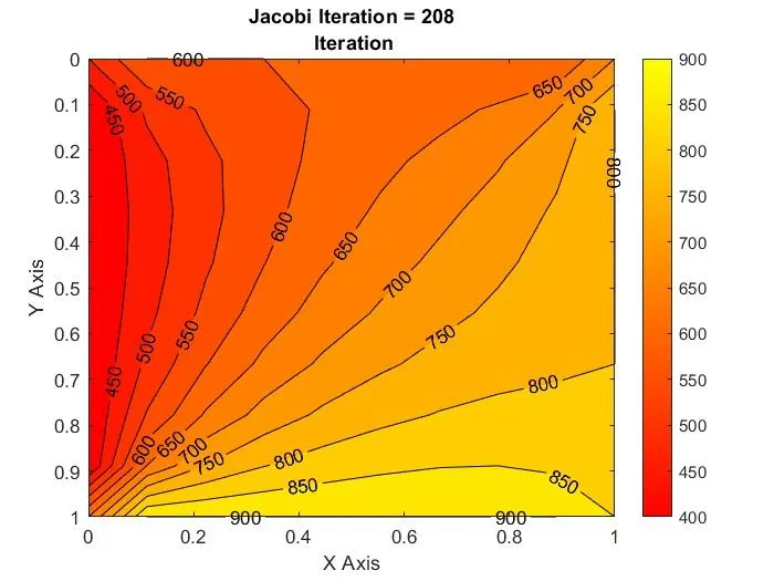
• Jacobi Method

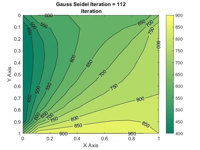
• Gauss-Seidel Method

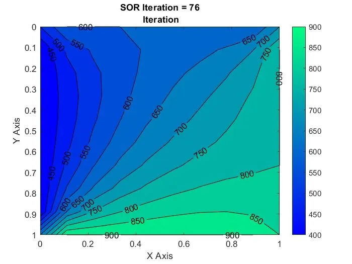
• SOR Method

Transient State Analysis

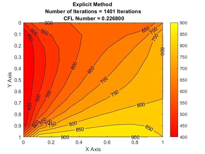
• Explicit Method

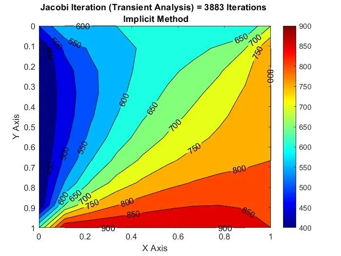
• Jacobi Method

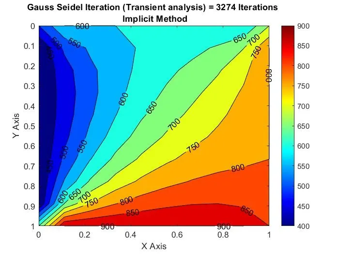
• Gauss-Seidel Method

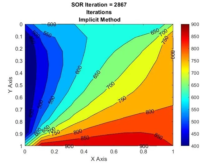
• SOR Method

CONCLUSION

1. The number of iterations for SOR is less compared to the other two methods.
2. The number of iterations --- Jacobian method > Gauss-Seiedel method > SOR method.
3. The Explicit approach in transient state analysis is done by taking values from the current time step. This makes it easier when compared to the Implicit method. But we need to be careful while choosing the time step as higher values of the time step will result in an unstable solution. Also, the value of the CFL number in both the x and y directions must be less than 0.5 for a stable solution.
4. The Implicit approach takes values from the next time step. It is a computationally challenging approach but allows us to use higher values of time steps and stable solutions.