Week 5.1 - Mid term project - Solving the steady and unsteady 2D heat conduction problem

AIM:

• To Solve the 2D Heat Conduction equation point iterative techniques using Matlab.

OBJECTIVE:

• The given Boundary Conditions are given below,
• Top Boundary = 600 K
• Bottom Boundary = 900 K
• Left Boundary = 400 K
• Right Boundary = 800 K

The following method to solve the 2D heat conduction using this methods,

• 1. Jacobi
• 2. Gauss-seidel
• 3. Successive over-relaxation.

PROCEDURE:

THEORY – 2D HEAT CONDUCTION.

• Two-Dimensional heat conduction is governed by a second order partial differential equation. A solution must satisfy the differential equation and the four boundary conditions.
• Numerical solutions are often referred to as being the explicit method or implicit method.

EXPLICIT METHOD.

• When a direct computation of the dependent variables can be made in terms of known quantities, the computational is said to be explicit.

IMPLICIT METHOD.

• When the dependent variables are defined by couple sets of equations, and either a matrix or iterative technique is needed to obtain the solution, the numerical method is called as implicit method.

ITERATIVE SOLVERS.

• In order to solve the dependent Variables, the following iterative solvers are used, they are
• JACOBI METHOD
• GAUSS SEIDEL METHOD
• SUCCESSIVE OVER RELAXATION.

JACOBI METHOD ( Bronshtein and Scmendyayev 1987)

• Jacobi method is a method of solving a matrix equation on a matrix that has no zero along its main diagonal.
• Each diagonal element is solved for and an approximation value is plugged in.
• This process is then iterated until it converges.
• Jacobi method can be derived by n equation in linear system of equation of Ax = B

If, in the i th equation,

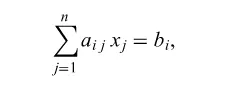
• Solve for value of `x_(i)`, while assuming other entries of x remains constant.

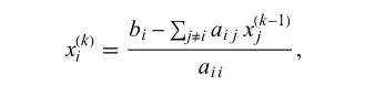
• In this method, the order in which equation are examined is irrelevant, since Jacobi method treats them independently.
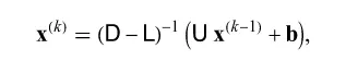
• The matrix form of Jacobi Method expressed as,

• Where, D is DIAGONAL,
• - L is LOWER TRIANGLE,
• U is strictly UPPER TRIANGLE.

GAUSS – SEIDEL METHOD.

• Gauss-Seidel method is a technique for solving the n equation of the linear system of equation Ax = B one at the time in the sequence, and uses previously computed results as soon as they are available.

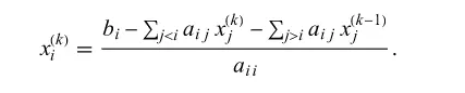
• There are two important characteristics of Gauss Seidel method should be noted.
• Firstly, the computational appear is serial.
• Since each component of new iterative depends upon all previously computed components, the updates cannot be done simultaneously as Jacobi Method.
• Secondly, the new iterative x(k) depends upon the order in which equations are examined. if this ordering is changed the components of new iterates (and not just orders) will also change.
• The matrix form of Gauss-Seidel method expressed as

• Where, D is DIAGONAL,
• - L is LOWER TRIANGLE,
• U is strictly UPPER TRIANGLE.

SUCCESSIVE OVER RELAXATION METHOD.

• Successive Over Relaxation method (SOR) is a technique for solving linear equation of Ax= B derived by extrapolating the Gauss – Seidel method.
• This extrapolation takes the form of a weighted average between the pervious iterate and the computed Gauss-Seidel iterate successively for each component.

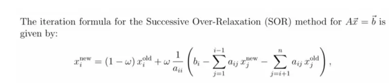
• Where x denotes Gauss- Seidel iterate, whereas `omega` is extrapolation factor.
• The idea is to choose the value for w that will accelerate the rate of convergence of iterates to solution.
• The matrix form of SOR method expressed as,

CONDUCTION.

• Conduction is the process by which heat is transformed from the hotter end to the colder end of an object. The ability of object to conduct heat is known as its thermal conducticity and is denoted by K.
• There are many conduction process, let us consider the following two process which is needed for this problem,

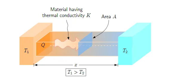One Dimensional Heat Conduction

STEADY STATE CONDUCTION.

TRANSIENT CONDUTION.

STEADY STATE CONDUCTION.

• Steady State conduction ids the form of conduction that happens when the temperature difference(s)driving the conduction are constant,so that (after an equilibrium time),the spatical distribution of temperature (temperature field) in the conducting object does noyt change any further.

3D HEAT CONDUCTION.

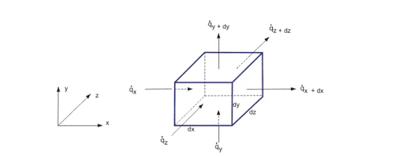
`(delT)/(delt) + alpha ( (del^2 T)/(delx^2) +(del^2T)/(dely^2) +(del^2T)/(delz^2)) = 0`

term 1 is time derivative whereas,

term 2 is the steady state flow.

LAPLACE EQUATION.

`((del^2T)/(delx^2) + (del^2T)/(dely^2) +(del^2T)/(delz^2) ) = grad^2T = 0`

In our problem let us govern the 2D heat conduction.

2D STEADY STATE HEAT CONDUCTION.

`(delT)/(delt) + alpha ((del^2T)/(delx^2) + (del^2T)/(dely^2)) = 0`

`((del^2T)/(delx^2) + (del^2T)/(dely^2) ) = 0`

With the help of Central Difference Scheme, Numerical Discretization is done.

CENTRAL DIFFERENCE SCHEME.

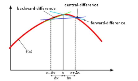
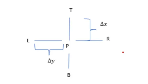
`(T_L-2T_P+T_R)/(delx^2) +(T_T -2T_P+T_B)/(dely^2) = 0`

`(2T_P)/(delx^2) +(2T_P)/(dely^2) = ((T_L+T_R)/(delx^2)) +((T_T+T_B)/(dely^2))`

• taking T_p common

`T_P ((2delx^2 +dely^2)/(delx^2*dely^2)) = ((T_L+T_R)/(delx^2) +(T_T+T_B)/(dely^2))`

`k = ((2delx^2+dely^2)/(delx^2*dely^2))`

`T_P = 1/k((T_L+T_R)/(delx^2) +(T_T+T_B)/(dely^2))`

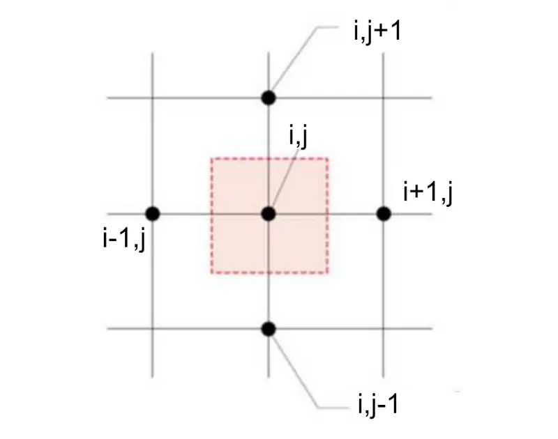
• The final equation is,

`T_(i j) = 0.25(T_(i-1),_j +T_(i+1),_j +T_(i,j+1) +T_(i,j-1)`

2D UNSTEADY / TRANSIENT HEAT CONDUCTION.

TRANSCIENT CONDUCTION.

• During any period in which temperature changes in time at any place within the object, the mode of thermal energy flow in termed as transient conduction.

EXPLICIT FORM.

`(delT)/(delt) = alpha((del^2T)/(delx^2) +(del^2T)/(dely^2))`

By discretization will get,

`(T_P^(n+1) -T_P)/(delt) = alpha((T_L-2T_P +T_R )/(delx^2) +(T_T-2T_P+T_B)/(dely^2))^n`

final expression

`T_P^(n+1) = T_p^n +k1(T_L-2T_P +T_R)^n +k2(T_T-2T_P+T_B)^n`

let

`k1 = alpha(delt)/(delx^2) ; k2 = alpha(delt)/(dely^2)`

For explicit we dont need iterative solvers, because there is only one unknown value.

IMPLICIT FORM.

`(delT)/(delt) =alpha ((del^2T)/(delx^2) +(del^2T)/(dely^2))`

Numerical discretization

`(T_P^(n+1) -T_P)/(delt) = alpha((T_L-2T_P+T_R)/(delx^2) +(T_T-2T_P+T_B)/(dely^2))^(n+1)`

`T_P^(n+1) = 1/(1+k1+k2) (T_P^n +k1(T_L+T_R)^(n+1) + k2(T_T+T_B)^(n+1))`

`k1 = alpha (delT)/(delx^2) ; k2 = alpha(delt)/(dely^2)`

BOUNDARY CONDITIONS.

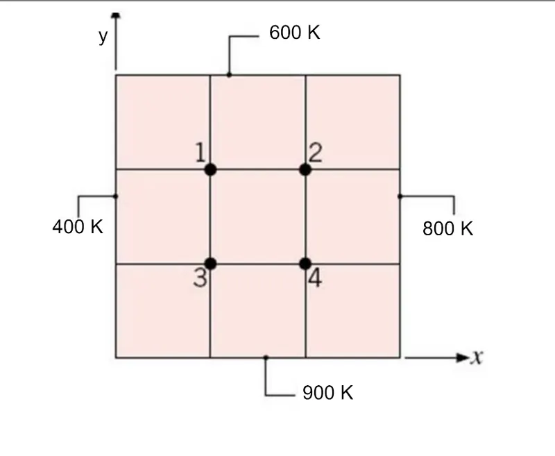
• Top Boundary = 600 K
• Bottom Boundary = 900 K
• Left Boundary = 400 K
• Right Boundary = 800 K

PESUCODE FUNCTION.

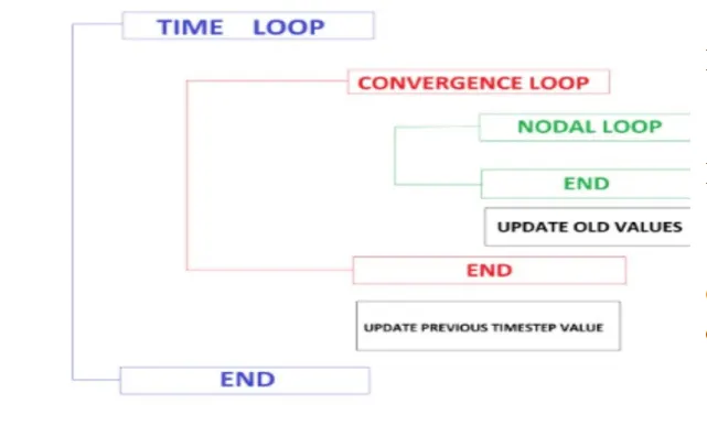
MAIN PROGRAM.

2D STEADY STATE CONDUCTION.

JACOBI METHOD.

% Solving Steady State 2d Heat Conduction Jacobi method.
clear all 
close all 
clc 

% Inputs 

% Length of the domain 
L = 1;
% Number of grid points in the x axis 
nx = 10;
% Number of grid points in the y axis 
ny = 10;

% Calculations 
x = linspace(0,L,nx);
y = linspace(0,L,ny);

dx = L/(nx-1);
dy = L/(ny-1);

% meshgrid 
[xx,yy] = meshgrid(x,y);

% Assuming the Error and Defining the Tolerance Value
error = 9e9;
tolerance = 1e-4;

% Initializing the Boundary Conditions 

% For Left Domain 400k
T_L = 400;
% For Right Domain 800k
T_R = 800;
% For Top Domain 600k
T_T = 600;
% For Bottom Domain 900k
T_B = 900;

% Initial Conditions
T = 300*ones(nx,ny);
T(2:ny-1,1) = T_L;
T(2:ny-1,nx) = T_R;
T(1,2:nx-1) = T_T;
T(ny,2:ny-1) = T_B;

% Calculating T average 
T(1,1)   = (T_L+T_T)/(2);
T(1,ny)  = (T_T+T_R)/(2);
T(nx,ny) = (T_R+T_B)/(2);
T(nx,1)  = (T_L+T_B)/(2);

T_initial = T;
T_old = T;
 

% JACOBI METHOD
iterative_solver=1;

if iterative_solver ==1
    jacobi_iter = 1;

    while (error>tolerance) 

        for i = 2:nx-1
            for j = 2:ny-1
                T(i,j) = 0.25*(T_old(i-1,j)+T_old(i+1,j)+T_old(i,j-1)+T_old(i,j+1));
            end
        end
        error = max(max(abs(T_old-T)));
        T_old = T;
        jacobi_iter = jacobi_iter+1;
    end
end

% Plotting

contourf(x,y,T)
clabel(contourf(x,y,T))
colorbar
colormap(jet)
set(gca,'ydir','reverse')
xlabel('x axis','FontSize',12)
ylabel('y axis','FontSize',12)
title(sprintf('No of JACOBI ITERATION =%d',jacobi_iter))
pause(0.03)

OUTPUT.

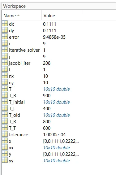
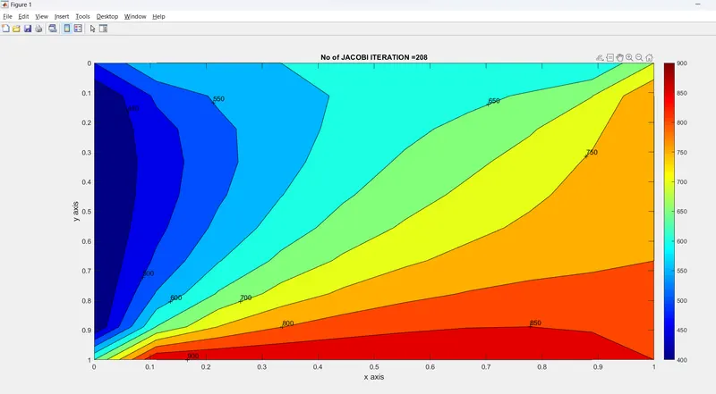
ERROR.

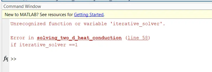
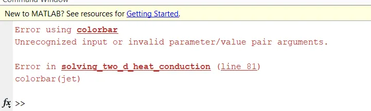
GAUSS SEIDEL METHOD.

% Solving 2d Heat Conduction Gauss Seidel Method 
clear all 
close all
clc 

% Inputs 

% Length of the domain 
L = 1;
% Number of grid points in the x axis 
nx = 10;
% Number of grid points in the y axis 
ny = 10;

% Calculations 
x = linspace(0,L,nx);
y = linspace(0,L,ny);

dx = L/(nx-1);
dy = L/(ny-1);

% meshgrid 
[xx,yy] = meshgrid(x,y);

% Assuming the Error and Defining the Tolerance Value
error = 9e9;
tolerance = 1e-4;

% Initializing the Boundary Conditions 

% For Left Domain 400k
T_L = 400;
% For Right Domain 800k
T_R = 800;
% For Top Domain 600k
T_T = 600;
% For Bottom Domain 900k
T_B = 900;

% Initial Conditions
T = 300*ones(nx,ny);
T(2:ny-1,1) = T_L;
T(2:ny-1,nx) = T_R;
T(1,2:nx-1) = T_T;
T(ny,2:ny-1) = T_B;

% Calculating T average 
T(1,1)   = (T_L+T_T)/(2);
T(1,ny)  = (T_T+T_R)/(2);
T(nx,ny) = (T_R+T_B)/(2);
T(nx,1)  = (T_L+T_B)/(2);

T_initial = T;
T_old = T;

% GAUSS SEIDEL METHOD
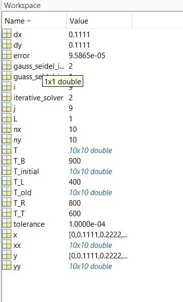
iterative_solver = 2;

if iterative_solver==2
    guass_seidel_iter = 1;
    
    while(error>tolerance)

    for i = 2:nx-1
        for j = 2:ny-1
            T(i,j) = 0.25*(T(i-1,j)+T_old(i+1,j)+T_old(i,j+1)+T(i,j-1));
        end
    end
    error = max(max(abs(T_old-T)));
    T_old = T;
    gauss_seidel_iter = guass_seidel_iter+1;
    end
end

% Plotting 
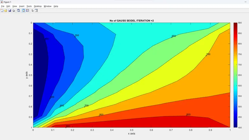
contourf(x,y,T)
clabel(contourf(x,y,T))
colorbar
colormap(jet)
set(gca,'ydir','reverse')
xlabel('x axis','FontSize',12)
ylabel('y axis','FontSize',12)
title(sprintf('No of GAUSS SEIDEL ITERATION =%d',gauss_seidel_iter))
pause(0.03)

OUTPUT.

SUCCESSIVE OVER RELAXATION.

% Solving 2d Heat Conduction Successive Over Relaxation Method 
clear all 
close all
clc 

% Inputs 

% Length of the domain 
L = 1;
% Number of grid points in the x axis 
nx = 10;
% Number of grid points in the y axis 
ny = 10;

% Calculations 
x = linspace(0,L,nx);
y = linspace(0,L,ny);

dx = L/(nx-1);
dy = L/(ny-1);

% meshgrid 
[xx,yy] = meshgrid(x,y);

% Assuming the Error and Defining the Tolerance Value
error = 9e9;
tolerance = 1e-4;
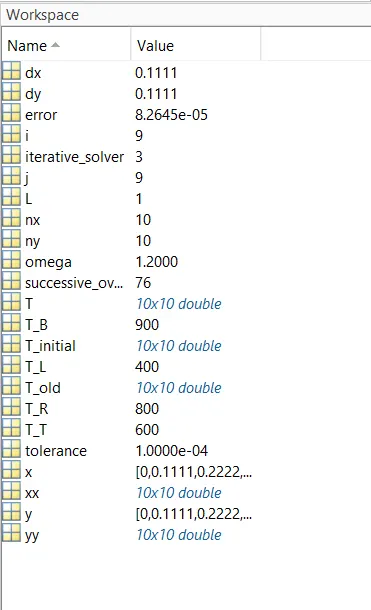
omega = 1.2;

% Initializing the Boundary Conditions 

% For Left Domain 400k
T_L = 400;
% For Right Domain 800k
T_R = 800;
% For Top Domain 600k
T_T = 600;
% For Bottom Domain 900k
T_B = 900;

% Initial Conditions
T = 300*ones(nx,ny);
T(2:ny-1,1) = T_L;
T(2:ny-1,nx) = T_R;
T(1,2:nx-1) = T_T;
T(ny,2:ny-1) = T_B;

% Calculating T average 
T(1,1)   = (T_L+T_T)/(2);
T(1,ny)  = (T_T+T_R)/(2);
T(nx,ny) = (T_R+T_B)/(2);
T(nx,1)  = (T_L+T_B)/(2);

T_initial = T;
T_old = T;

% SUCCESSIVE OVER RELAXATION METHOD
iterative_solver = 3;

if iterative_solver==3
    successive_over_relaxation_iter = 1;
    
    while(error>tolerance)

    for i = 2:nx-1
        for j = 2:ny-1
            T(i,j) = omega*(0.25*(T(i-1,j)+T_old(i+1,j)+T_old(i,j+1)+T(i,j-1)))+(1-omega)*T_old(i,j);
        end
    end
    error = max(max(abs(T_old-T)));
    T_old = T;
    successive_over_relaxation_iter = successive_over_relaxation_iter+1;
    end
end

% Plotting 
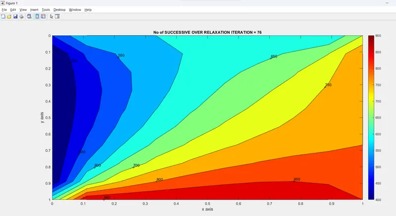
contourf(x,y,T)
clabel(contourf(x,y,T))
colorbar
colormap(jet)
set(gca,'ydir','reverse')
xlabel('x axis','FontSize',12)
ylabel('y axis','FontSize',12)
title(sprintf('No of SUCCESSIVE OVER RELAXATION ITERATION = %d',successive_over_relaxation_iter))
pause(0.03)

OUTPUT.

PROGRAM.

2D UNSTEADY STATE CONDUCTION.

EXPLICIT METHOD.

% Solving Unsteady State Heat Condduction Explicit Method
clear all 
close all 
clc

% Inputs 
% length of the domain 
L = 1;
% Number of grids in x axis 
nx= 10;
% Number of grids in y axis 
ny = 10;

% time marching 
nt = 1400;

x = linspace(0,L,nx);
y = linspace(0,L,ny);


dx = L/(nx-1);
dy = L/(ny-1);

% Assuming and defining error values,tolerance,omega 
error = 9e9;
tolerance = 1e-4;
dt = 1e-5;
omega = 1.1;

% Initializing boundary conditions and initial conditions 
T_L = 400;
T_R = 800;
T_T = 600;
T_B = 900;

T=300*ones(nx,ny);
T(2:ny-1,1)  = T_L;
T(2:ny-1,nx) = T_R;
T(1,2:nx-1)  = T_T;
T(ny,2:ny-1) = T_B;

% Calculating T average 
T(1,1) = (T_L+T_T)/(2);
T(nx,ny)= (T_R+T_B)/(2);
T(1,ny) = (T_T+T_R)/(2);
T(nx,1) = (T_L+T_B)/(2);

T_initial = T;
T_old = T;

% Explicit method 

k1 = 1.1*((dt)/(dx^2));
k2 = 1.1*((dt)/(dy^2));

iterative_solver = 1;

if iterative_solver==1
   unsteady_explicit_iter = 1;
    for k = 1:nt
        error= 9e9;
        while(error>tolerance)
            for i = 2:nx-1
                for j = 2:ny-1

                    term1= T_old(i,j);
                    term2= k1*(T_old(i+1,j)-2*T_old(i,j)+(T_old(i-1,j)));
                    term3 = k2*(T_old(i,j+1)-2*T_old(i,j)+(T_old(i,j-1)));
                    T(i,j)= term1+term2+term3;
                end
            end
            error= max(max(abs(T_old-T)));
            T_old = T;
            unsteady_explicit_iter= unsteady_explicit_iter+1;
        end
    end
end
 % Plotting 
   contourf(x,y,T)
   clabel(contourf(x,y,T))
   colorbar
   colormap(jet)
   set(gca,'ydir','reverse')
   xlabel('X axis','FontSize',14)
   ylabel('Y axis','FontSize',14)
   title(sprintf('NO OF UNSTEADY HEAT CONDUCTION ITERATION (EXPLICIT)=%d',unsteady_explicit_iter));
   pause(0.003)

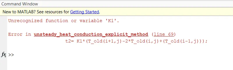
ERROR.

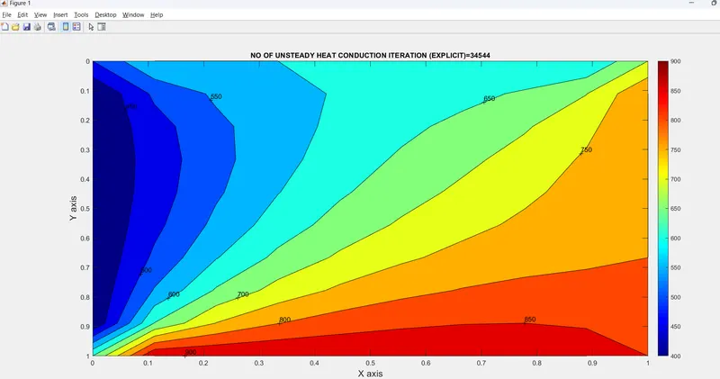
OUTPUT.

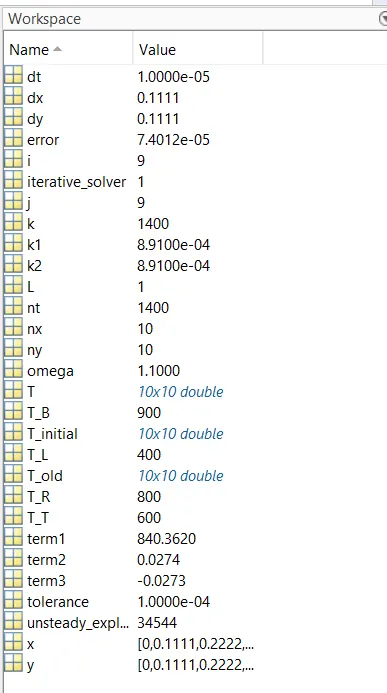
• When assuming dt = 1e-2; couldn't able to get the term1,term2 term3 values, instead the value of dt = 1e-5. (explicit )

2D UNSTEADY STATE CONDUCTION.

IMPLICIT METHOD.

JACOBI METHOD.

% solving Unsteady Heat conduction Using jacobi Method(IMPLICIT)
clear all 
close all 
clc 

% Inputs
% length of the domain 
L = 1;
% Number of grid points in the x axis 
nx = 10;
% Number of grid points in the y axis 
ny = 10;
% time marching 
nt = 1400;

% Calculations 
x = linspace(0,L,nx);
y = linspace(0,L,ny);

dx = L/(nx-1);
dy = L/(ny-1);

% meshgrid 
[xx,yy] = meshgrid(x,y);

% Assuming the Error,dt and Defining the Tolerance Value
error = 9e9;
tolerance = 1e-4;
dt = 1e-2;

% Initializing the Boundary Conditions 

% For Left Domain 400k
T_L = 400;
% For Right Domain 800k
T_R = 800;
% For Top Domain 600k
T_T = 600;
% For Bottom Domain 900k
T_B = 900;

% Initial Conditions
T = 300*ones(nx,ny);
T(2:ny-1,1) = T_L;
T(2:ny-1,nx) = T_R;
T(1,2:nx-1) = T_T;
T(ny,2:ny-1) = T_B;

% Calculating T average 
T(1,1)   = (T_L+T_T)/(2);
T(1,ny)  = (T_T+T_R)/(2);
T(nx,ny) = (T_R+T_B)/(2);
T(nx,1)  = (T_L+T_B)/(2);

T_initial = T;
T_old = T;

% calculating 2d unsteady heat conduction for jacobi method
k1 = 1.1*(dt/(dx^2));
k2 = 1.1*(dt/(dy^2));

% creating movie 
ct =1;

jacobi_iter = 1;

% time loop 
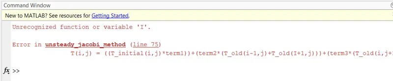
for k = 1:nt 
    error = 9e9;
    while(error>tolerance)
        for i = 2:nx-1
            for j = 2:ny-1
                term1= 1/(1+2*k1+2*k2);
                term2 = k1*term1;
                term3 = k2*term1;
                T(i,j) = ((T_initial(i,j)*term1))+(term2*(T_old(i-1,j)+T_old(i+1,j)))+(term3*(T_old(i,j+1)+T_old(i,j-1)));
            end
        end
  
        error = max(max(abs(T_old-T)));
        T_old = T;
        jacobi_iter = jacobi_iter+1;
    end

    T_initial = T;

    % plotting 
    contourf(x,y,T)
    clabel(contourf(x,y,T))
    colorbar
    colormap(jet)
    set(gca,'ydir','reverse')
    xlabel('X axis','FontSize',14)
    ylabel('Y axis','FontSize',14)
    title(sprintf('No Of JACOBI ITERATION(IMPLICIT)=%d',jacobi_iter));
    pause(0.003)
    M(ct)= getframe(gcf);
    ct = ct+1;
end

movie(M)
videofile = VideoWriter('Jacobi.avi','Uncompressed AVI');
open(videofile)
writeVideo(videofile,M)
close(videofile)

OUTPUT.

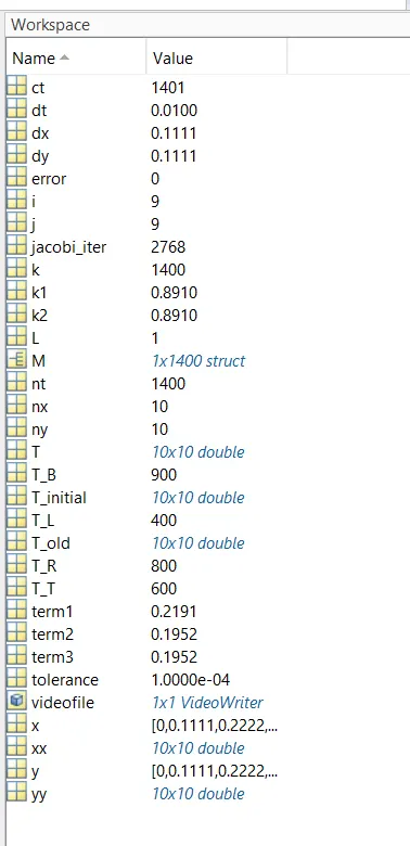
ERROR

GAUSS SEIDEL METHOD.

% solving Unsteady Heat conduction Using Gauss Seidel Method(IMPLICIT)
clear all 
close all 
clc 

% Inputs
% length of the domain 
L = 1;
% Number of grid points in the x axis 
nx = 10;
% Number of grid points in the y axis 
ny = 10;
% time marching 
nt = 1400;

% Calculations 
x = linspace(0,L,nx);
y = linspace(0,L,ny);

dx = L/(nx-1);
dy = L/(ny-1);

% meshgrid 
[xx,yy] = meshgrid(x,y);

% Assuming the Error,dt and Defining the Tolerance Value
error = 9e9;
tolerance = 1e-4;
dt = 1e-2;

% Initializing the Boundary Conditions 

% For Left Domain 400k
T_L = 400;
% For Right Domain 800k
T_R = 800;
% For Top Domain 600k
T_T = 600;
% For Bottom Domain 900k
T_B = 900;

% Initial Conditions
T = 300*ones(nx,ny);
T(2:ny-1,1) = T_L;
T(2:ny-1,nx) = T_R;
T(1,2:nx-1) = T_T;
T(ny,2:ny-1) = T_B;

% Calculating T average 
T(1,1)   = (T_L+T_T)/(2);
T(1,ny)  = (T_T+T_R)/(2);
T(nx,ny) = (T_R+T_B)/(2);
T(nx,1)  = (T_L+T_B)/(2);

T_initial = T;
T_old = T;


% calculating 2d unsteady heat conduction for jacobi method
k1 = 1.1*(dt/(dx^2));
k2 = 1.1*(dt/(dy^2));

% creating movie 
ct=1;
jacobi_iter = 1;

% time loop 
for k = 1:nt 
    error = 9e9;
    while(error>tolerance)
        for i = 2:nx-1
            for j = 2:ny-1
                term1= 1/(1+2*k1+2*k2);
                term2 = k1*term1;
                term3 = k2*term1;
                T(i,j) = ((T_initial(i,j)*term1))+(term2*(T(i-1,j)+T_old(i+1,j)))+(term3*(T(i,j+1)+T_old(i,j-1)));
            end
        end
  
        error = max(max(abs(T_old-T)));
        T_old = T;
        jacobi_iter = jacobi_iter+1;
    end

    T_initial = T;
 
   % Plotting 
   contourf(x,y,T)
   clabel(contourf(x,y,T))
   colorbar
   colormap(jet)
   set(gca,'ydir','reverse')
   xlabel('X axis','FontSize',14)
   ylabel('Y axis','FontSize',14)
   title(sprintf('No Of GAUSS SEIDEL ITERATION(IMPLICIT)=%d',jacobi_iter));
   pause(0.003)
   M(ct)=getframe(gcf);
   ct = ct+1;
    
end

movie(M)
videofile = VideoWriter('Gauss_seidel.avi','Uncompressed AVI');
open(videofile)
writeVideo(videofile,M)
close(videofile)

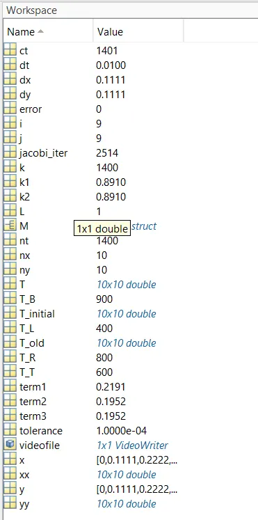
OUTPUT.

SUCCESSIVE OVER RELAXATION.

% solving Unsteady Heat conduction Using Successive Over Relaxation Method(IMPLICIT)
clear all 
close all 
clc 

% Inputs
% length of the domain 
L = 1;
% Number of grid points in the x axis 
nx = 10;
% Number of grid points in the y axis 
ny = 10;
% time marching 
nt = 1400;

% Calculations 
x = linspace(0,L,nx);
y = linspace(0,L,ny);

dx = L/(nx-1);
dy = L/(ny-1);

% meshgrid 
[xx,yy] = meshgrid(x,y);

% Assuming the Error,omega, dt and Defining the Tolerance Value
error = 9e9;
tolerance = 1e-4;
dt = 1e-2;
omega = 1.1;

% Initializing the Boundary Conditions 

% For Left Domain 400k
T_L = 400;
% For Right Domain 800k
T_R = 800;
% For Top Domain 600k
T_T = 600;
% For Bottom Domain 900k
T_B = 900;

% Initial Conditions
T = 300*ones(nx,ny);
T(2:ny-1,1) = T_L;
T(2:ny-1,nx) = T_R;
T(1,2:nx-1) = T_T;
T(ny,2:ny-1) = T_B;

% Calculating T average 
T(1,1)   = (T_L+T_T)/(2);
T(1,ny)  = (T_T+T_R)/(2);
T(nx,ny) = (T_R+T_B)/(2);
T(nx,1)  = (T_L+T_B)/(2);

T_initial = T;
T_old = T;
T_end = T;

% calculating 2d unsteady heat conduction for jacobi method
k1 = 1.1*(dt/(dx^2));
k2 = 1.1*(dt/(dy^2));

ct = 1;
gauss_seidel_iter = 1;
% time loop 
for k = 1:nt
    error = 9e9;
    while(error>tolerance)
        for i = 2:nx-1
            for j = 2:ny-1
                term1= 1/(1+2*k1+2*k2);
                term2 = k1*term1;
                term3 = k2*term1;
                T(i,j) = ((T_initial(i,j)*term1))+(term2*(T(i-1,j)+T_old(i+1,j)))+(term3*(T(i,j+1)+T_old(i,j-1)));
                T_end(i,j)= (1-omega)*(T_old(i,j))+(T(i,j)*omega);
            end
        end
        error= max(max(abs(T_old-T)));
        T_old = T_end;
        gauss_seidel_iter = gauss_seidel_iter+1;
    end
    T_initial= T_end;

   % Plotting 
   contourf(x,y,T)
   clabel(contourf(x,y,T))
   colorbar
   colormap(jet)
   set(gca,'ydir','reverse')
   xlabel('X axis','FontSize',14)
   ylabel('Y axis','FontSize',14)
   title(sprintf('No Of SUCCESSIVE OVER RELAXATION ITERATION(IMPLICIT)=%d',gauss_seidel_iter));
   pause(0.003)
   M(ct)=getframe(gcf);
   ct = ct+1;

end

movie(M)
videofile = VideoWriter('Successive_over_relaxation.avi','Uncompressed AVI');
open(videofile)
writeVideo(videofile,M)
close(videofile)

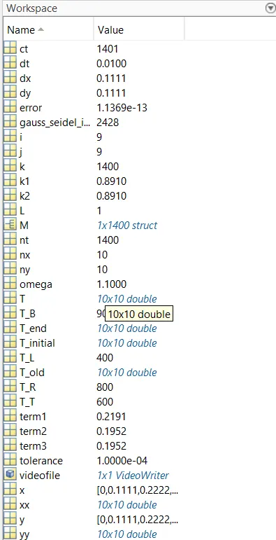
OUTPUT.

CODE EXPLANATION.

• The following program start's clear all close all clc commands respectively.
• clear all command is used to clear all the variables from the workspace,whereas the close all command is used to close the plots from the figure window.
• clc command is used to clear all the commands in the command window.
• The input parameters are given respectively(that is) the assuming length of the domain 1m; nx=ny =10;
• Linspace command is used to calculate the grid points of x and y axis respectively.
• After that meshgrid is used which tranforms the domain specified by the vectors into arrays.
• Initializing boundary conditions( errors,omega tolerance,time marching )values.
• T average is been calculated.with all of the inputs parameters space,time,converge loop are calculated with respect to iteration methods(Jacobi,Gauss Seidel,Successive OverRelaation) for both steady and Unsteady heat condution (Implicit method).
• ERROR values is also calculated inside the loop. Also for Unsteady method the plotting is done inside the loop.
• contourf( Z ) creates a filled contour plot containing the isolines of matrix Z , where Z contains height values on the x-y plane.Colo automatically selects the contour lines to display. The column and row indices of Z are the x and y coordinates in the plane, respectively.
• Colorbar allows to see the relationship between the data and colors displayed in the chart.
• Colormap is the matrix of values that defines the colors of graphite object such as surface,images and patch objects.
• sprintf command is used to translates escape-character sequences in literalText.

CONCLUSION.

• Let us conclude that Steady state analysis and Transient analysis is been calculated with respect to their inputs parameters and the follwing results are satisfied.