Week 5.1 - Mid term project - Solving the steady and unsteady 2D heat conduction problem

%2d heat conduction equation

clear all
close all
clc

%parameters needed
nx=10;
ny=10;
x=linspace(0,1,nx);
y=linspace(0,1,ny);
dx=x(2)-x(1);
dy=y(2)-y(1);
[xx,yy] = meshgrid(x,y);

%boundary conditions
T=ones(nx,ny);
T(1,:)=900;
T(end,:)=600;
T(:,1)=400;
T(:,end)=800;
Told=T;
et=1e-4;
se=9e9;

k=2*((dx^2+dy^2)/(dx^2*dy^2));

%code
iterative_solver = input('iterative solver:\');
if iterative_solver==1
    tic;
    T_jacobi= jacobi_iter(se,et,xx,yy,nx,ny,dx,dy,T,k,Told);
    toc
elseif iterative_solver==2
    tic;
    T_gauss= gauss_iter(se,et,xx,yy,nx,ny,dx,dy,T,k,Told);
    toc
elseif iterative_solver==3
    tic;
    T_sor= sor_iter(se,et,xx,yy,nx,ny,dx,dy,T,k,Told);
    toc
end


%function for jacobi method
function jacobi= jacobi_iter(se,et,xx,yy,nx,ny,dx,dy,T,k,Told)
     
     jacobi_iter=1;
     while(se > et)
     for i=2:nx-1
         for j=2:ny-1
          T(i,j) = (Told(i-1,j)+Told(i+1,j))/(k*(dx^2))+(Told(i,j-1)+Told(i,j+1))/(k*(dy^2));
         end
     end
     se=max(max(abs(Told-T)));
     Told=T;
     jacobi_iter=jacobi_iter+1;
     jacobi = figure(1)  
     [c,d]=contourf(xx,yy,T);
     colorbar
     tt=sprintf('Jacobi iteration(steady state) =%d',jacobi_iter);
     title(tt)
     xlabel('x axis')
     ylabel('y axis')
     clabel(c,d)
     pause(0.03)
     end
     fprintf(' Iterations =%d',jacobi_iter);
end

%function for gauss seidal method
function gauss_seidal= gauss_iter(se,et,xx,yy,nx,ny,dx,dy,T,k,Told)
     gs_iter=1;
   
     while(se > et)
     for i=2:nx-1
         for j=2:ny-1
         T(i,j)=(((T(i-1,j)+Told(i+1,j))/dx^2)+((T(i,j-1)+Told(i,j+1))/dy^2))/k;
         end
     end
     se=max(max(abs(Told-T)));
     Told=T;
     gs_iter=gs_iter+1;
     gauss_seidal=figure(2)   
     [c,d]=contourf(xx,yy,T);
     colorbar
     tt=sprintf('Gauss seidal iteration(steady state)=%d',gs_iter);
     title(tt)
     xlabel('x axis')
     ylabel('y axis')
     clabel(c,d)
     pause(0.03)
     end
     fprintf('Iterations=%d',GS_iter);
end

%function for successive over relaxation method
function sor= sor_iter(se,et,xx,yy,nx,ny,dx,dy,T,k,Told)
     sor_iter=1;
     alpha=1.2;
     
     while(se > et)
     for i=2:nx-1
         for j=2:ny-1
         T_gs=(((T(i-1,j)+Told(i+1,j))/dx^2)+((T(i,j-1)+Told(i,j+1))/dy^2))/k;
         T(i,j)= alpha*(T_gs)+(1-alpha)*(Told(i,j));
         end
     end
     se=max(max(abs(Told-T)));
     Told=T;
     sor_iter=sor_iter+1;
     sor = figure(3)   
     [c,d]=contourf(xx,yy,T);
     colorbar
     tt=sprintf('SOR iteration(steady state)=%d',sor_iter);
     title(tt)
     xlabel('x axis')
     ylabel('y axis')
     clabel(c,d)
     pause(0.03)
     end
     fprintf('Iterations=%d',sor_iter);
end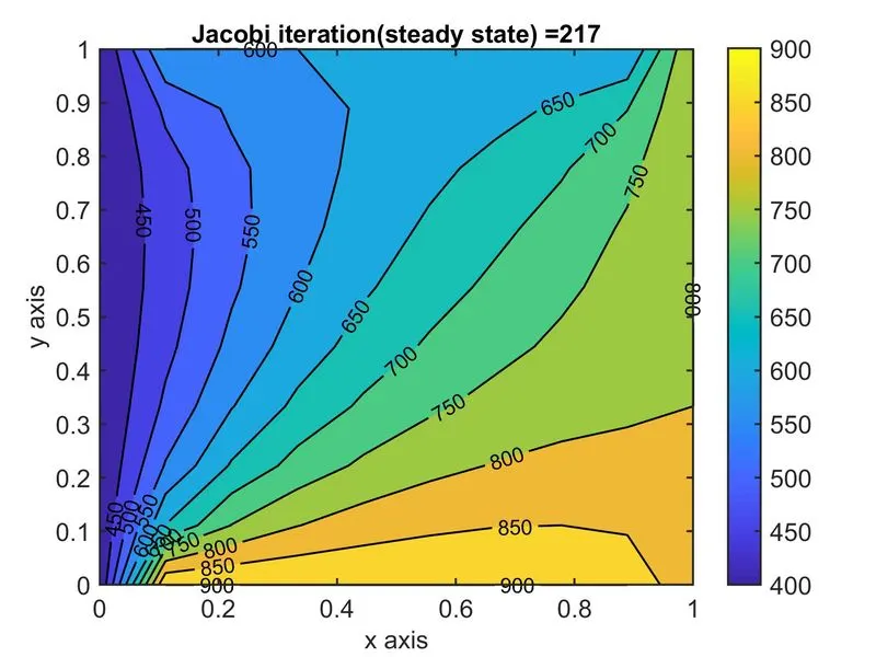

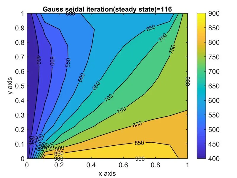
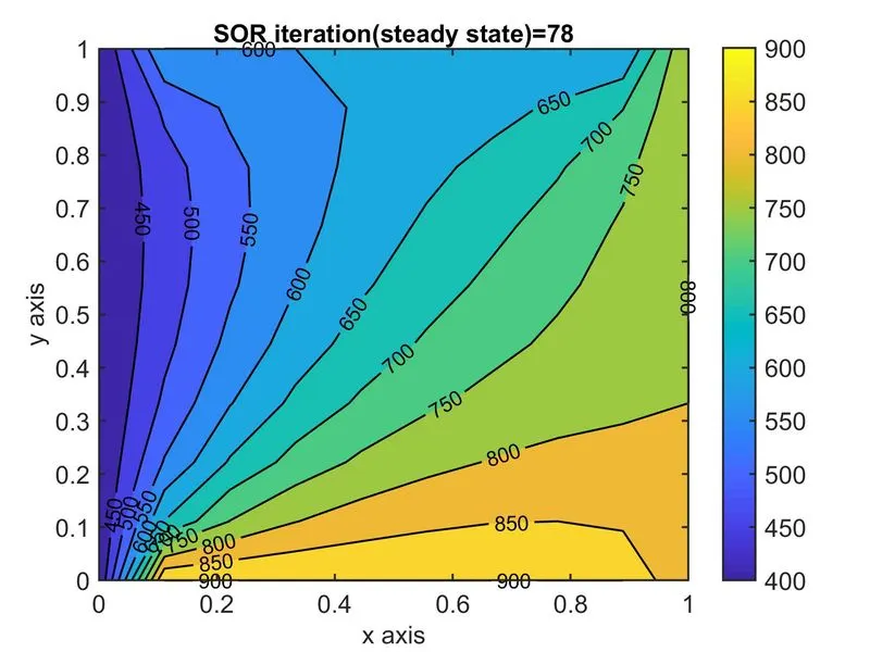
Here, steady state analysis for the 2D heat conduction equation is done. For this, the point iterative techniques used are Jacobi method, Gauss-seidal method, and successive over relaxation method. First, we write a program for the steady state condition with the provided boundary conditions. At first, we define all the parameters required like the number of nodes in x and y direction, grid spacing, and convert them in to an array using meshgrid command. Then, we specify the boundary conditions required such as the temperatures at the top, bottom, left and right, and create an array with respect to the dimensions of nx and ny, and set all the values as 1. Then we define the absolute error, starting error, and value for k. Then, we can initiate a loop where the code is executed only if the value matches the input obtained from the end user, i.e. 1 for jacobi, 2 for gauss seidal and 3 for sor method. If the value matches, the code runs and an if loop is executed inside which the jacobi, gauss seidal or the sor functions are run depending upon the value obtained from the end user.

For writing the functions of jacobi, gauss seidal and sor methods, we create a function for the dependent variables, set the iteration initial at 1, and execute a while loop with condition where the loop is executed only if the value for the starting error is greater than that of the absolute error. If the condition is satisfied, then there are two for loops where the iterations run from 2 to the values of nx and ny -1 respectively, and the formula for the particular method is executed. AFter the loop is run, the error value for starting error is set to the latest calculated value, old values are assigned to the temperature matrix, and the iteration is incremented each time the loop is executed. Then, we plot the graph using contour plot, count the number of iterations run, provide appropriate labels and titles, and get the values for iterations and time run.

%2d heat condn equation transcient implicit method
clear all
close all
clc

%parameters needed
nx=10;
ny=10;
L=1;
x=linspace(0,1,nx);
y=linspace(0,1,ny);
dx=x(2)-x(1);
dy=y(2)-y(1);
dt=0.01;
alpha=2e-5;
[xx,yy] = meshgrid(x,y);

%defining the boundary conditions
T=ones(nx,ny);
T(1,:)=900;
T(end,:)=600;
T(:,1)=400;
T(:,end)=800;
%rounding off the corner value by taking the average value
T(1,1) = (400+900)/2;
T(1,ny) = (900+800)/2;
T(nx,1) = (400+600)/2;
T(nx,ny) = (600+800)/2;
Told=T;
Tprev=Told;
et=1e-4;
se=9e9;
k1= alpha*(dt/(dx^2));
k2= alpha*(dt/(dy^2));
beta=2/(1+sin(pi*dx));
CFL= alpha*(dt/(dx^2));

%code
iterative_solver = input('Iterative solver');
if iterative_solver==1
    tic;
    T=jacobi_iter_trans_impli(se,et,xx,yy,nx,ny,T,k1,k2,Told,Tprev);
elseif iterative_solver==2
    tic;
    T_gs= gs_iter_trans_impli(se,et,xx,yy,nx,ny,T,k1,k2,Told,Tprev);
elseif iterative_solver==3
    tic;
    T_sor= sor_iter_trans_impli(se,et,xx,yy,nx,ny,T,k1,k2,Told,Tprev,beta);
end

%function for jacobi method (transcient implicit)    
function   jti=jacobi_iter_trans_impli(se,et,xx,yy,nx,ny,T,k1,k2,Told,Tprev)   
    jacobi_iter=1; 
for k= 1:100
    se=9e9;
     while(se > et)
     for i=2:nx-1
         for j=2:ny-1
          T(i,j)= (Tprev(i,j)*(1+(2*k1)+(2*k2))^(-1))+k1*(1+(2*k1)+(2*k2))^(-1)*(Told(i-1,j)+Told(i+1,j))+k2*(1+(2*k1)+(2*k2))^(-1)*(Told(i,j-1)+Told(i,j+1));
         end
     end
     se=max(max(abs(Told-T)));
     Told=T;
     jacobi_iter=jacobi_iter+1; 
     end
    Tprev=T;
end
     jti = figure(1)
     time_jacobi=toc;
     contourf(xx,yy,T)
     colorbar
     xlabel('x axis')
     ylabel('y axis')
     colorbar
     tt=sprintf('Jacobi Iteration=%d and time=%f sec',jacobi_iter,time_jacobi);
     title(tt)
     fprintf('Iteration=%d time (sec)=%f',jacobi_iter,time_jacobi);
end

%function for GS method (transcient implicit)
function gsti= gs_iter_trans_impli(se,et,xx,yy,nx,ny,T,k1,k2,Told,Tprev)
 gs_iter=1;
for k=1:100
         se=9e9;
    while(se > et)  
     for i=2:nx-1
         for j=2:ny-1
          T(i,j)= Tprev(i,j)*(1+(2*k1)+(2*k2))^-1+k1*(1+(2*k1)+(2*k2))^-1*(T(i-1,j)+Told(i+1,j))+k2*(1+(2*k1)+(2*k2))^-1*(T(i,j-1)+Told(i,j+1));
         end
     end
     se=max(max(abs(Told-T)));
     Told=T;
     gs_iter=gs_iter+1; 
    end
    Tprev=T;
end
    gsti = figure(2)
    time_gs=toc;
    contourf(xx,yy,T)
    colorbar
    xlabel('x axis')
    ylabel('y axis')
    colorbar
    tt=(sprintf(' Gauss seidal iteration=%d time=%f sec',gs_iter,time_gs));
    title(tt)
    fprintf('Iteration=%d time (sec)=%f',gs_iter,time_gs);
end

%function for SOR method (transcient implicit)
function T=sor_iter_trans_impli(se,et,xx,yy,nx,ny,T,k1,k2,Told,Tprev,beta)
     sor_iter=1;
 for k=1:100
     se=9e9;
    while(se > et)
     for i=2:nx-1
         for j=2:ny-1
          T(i,j)= beta*(Tprev(i,j)*(1+(2*k1)+(2*k2))^-1+k1*(1+(2*k1)+(2*k2))^-1*(T(i-1,j)+Told(i+1,j))+k2*(1+(2*k1)+(2*k2))^-1*(T(i,j-1)+Told(i,j+1)))+(1-beta)*Tprev(i,j);
         end
     end
     se=max(max(abs(Told-T)));
     Told=T;
     sor_iter=sor_iter+1; 
    end
     Tprev=T;
 end
     time_sor=toc;
     contourf(xx,yy,T)
     colorbar
     xlabel('x axis')
     ylabel('y axis')
     colorbar
     tt=(sprintf('SOR iteration=%d time=%f sec',sor_iter,time_sor));
     title(tt)
     fprintf('Iteration=%d time=%f',sor_iter,time_sor);
    
end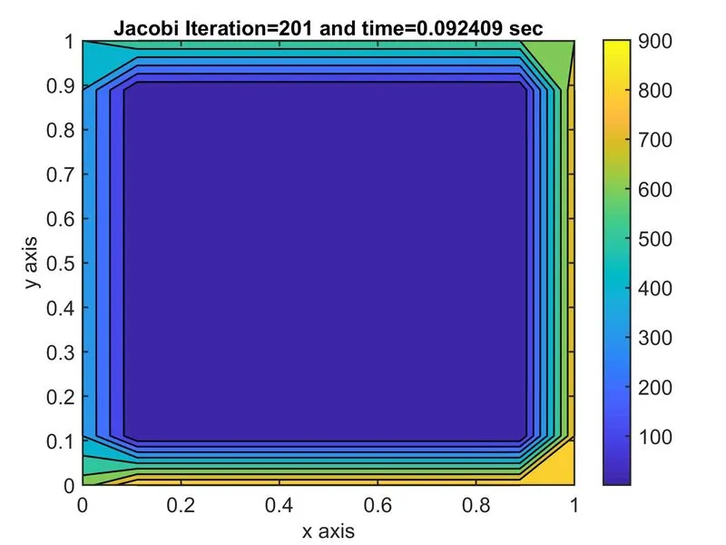

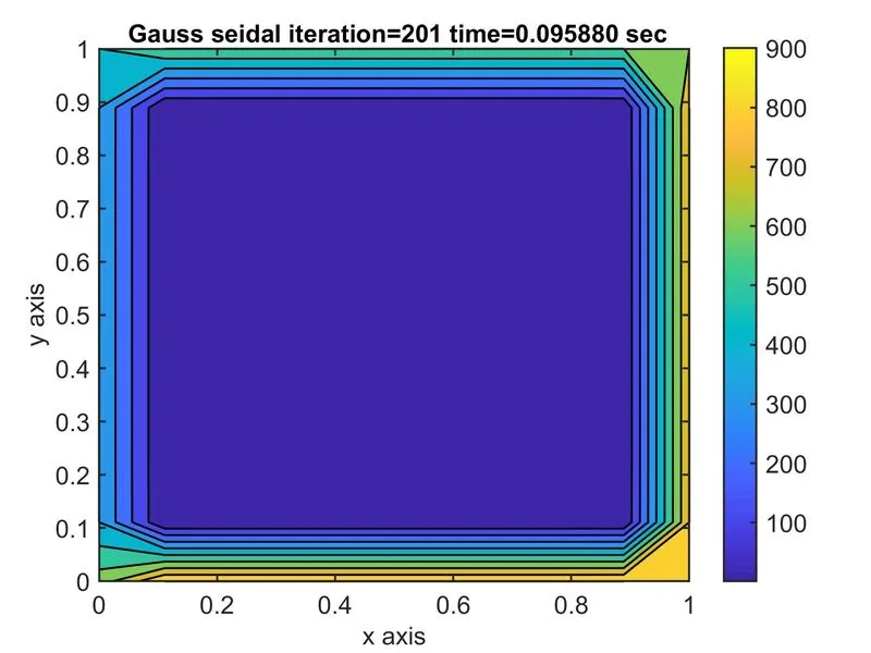
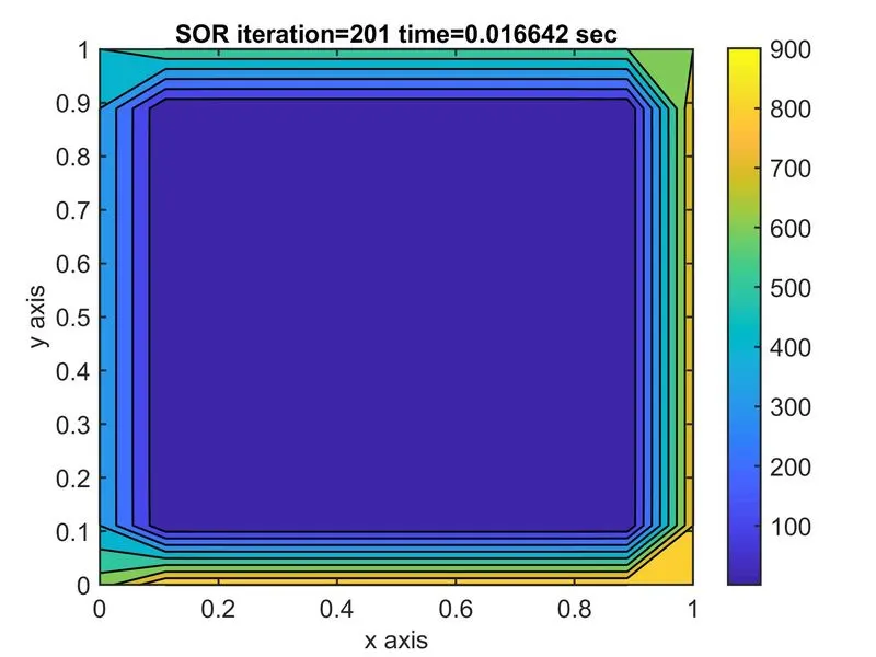
Similarly, for the Transcient-implicit method, program is written where the function for each point iterative techniques are called according to the value entered by end user and each functions are separately written but here, the value of itertaions are fixed to 100.

%2d heat condn equation trasncient explicit method
clear all
close all
clc

%parameters needed
nx=10;
ny=10;
x=linspace(0,1,nx);
y=linspace(0,1,ny);
dx=x(2)-x(1);
dy=y(2)-y(1);
dt=0.01;
alpha=2e-5;
[xx,yy] = meshgrid(x,y);

%defining the boundary conditions
T=ones(nx,ny);
T(1,:)=900;
T(end,:)=600;
T(:,1)=400;
T(:,end)=800;
Told=T;
T(1,1) = (400+900)/2;
T(1,ny) = (900+800)/2;
T(nx,1) = (400+600)/2;
T(nx,ny) = (600+800)/2;
et=1e-4;
se=9e9;
k1= alpha*(dt/dx^2);
k2= alpha*(dt/dy^2);

%code
iterative_solver = 1;
tic;
if iterative_solver==1
    T_jacobi= jacobi_iter_trasient(xx,yy,nx,ny,T,k1,k2,Told);
end
toc


%function for jacobi method transcient(explicit)
function jte= jacobi_iter_trasient(xx,yy,nx,ny,T,k1,k2,Told)
     jacobi_iter=1;
    for k=1:100
     for i=2:nx-1
         for j=2:ny-1
          T(i,j) = Told(i,j)+k1*(Told(i+1,j)-2*Told(i,j)+Told(i-1,j))+k2*(Told(i,j+1)-2*Told(i,j)+Told(i,j-1)) ;
         end
     end
     se=max(max(abs(Told-T)));
     Told=T;
     jacobi_iter=jacobi_iter+1;
    end
     jte=figure(1)  
     [c,d]=contourf(xx,yy,T);
     colorbar
     title_text=sprintf('Jacobi iteration (Transcient explicit)=%d',jacobi_iter);
     title(title_text)
     xlabel('x axis')
     ylabel('y axis')
     clabel(c,d)
     pause(0.03)
     fprintf('Iterations=%d',jacobi_iter);
    
end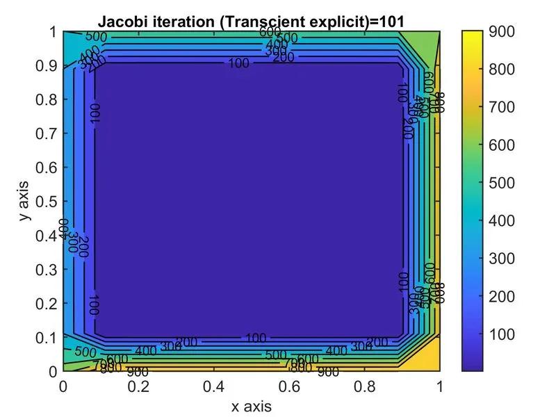

Finally, program for solving the 2D heat conduction equation using jacobi point iterative method explicitely is written and the plots are obtained in a similar manner. From the results obtained, it is evident that for the SOR method, the time taken to run is much less than the other two methods,and takes less number of iterations, where as jacobi method takes the most time and number of iterations is also higher comparitively therefore, SOR method can be preffered while solving steady state equations where higher efficiency is required. Secondly, the time for solving the equation using transcient method is more therefore, using steady state conditions to solve can be done and using explicit method, which is quicker can be more efficient only when the courant number is <0.25. Finally, for the implicit transcient condition, jacobi method takes the least time to run and the result obtained from the SOR method is the stable one.