Week 5.1 - Mid term project - Solving the steady and unsteady 2D heat conduction problem
Solving the steady and unsteady 2D heat conduction problem
Aim: To solve the 2D heat conduction equation by using the point iterative techniques (Steady state analysis & Transient State Analysis)
Given Problem:
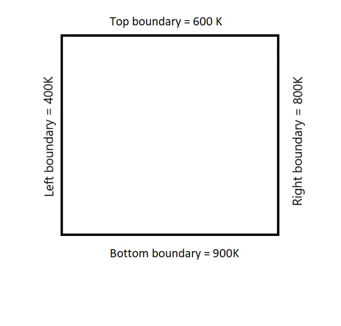
The Boundary conditions for the problem are as follows;
Top Boundary = 600 K
Bottom Boundary = 900 K
Left Boundary = 400 K
Right Boundary = 800 K
For Steady State heat conduction:
`((del^2T)/(delx^2) + (del^2T)/(dely^2)) = 0`
Now in order to solve the above governing equation we first discretize the equation by using a central differencing scheme which is as follows:
`(Toverset(n)(underset(i+1,j)())-2Toverset(n)underset(i,j)()+Toverset(n)underset(i-1,j)())/(trianglex^2)+(Toverset(n)underset(i,j+1)()-2Toverset(n)underset(i,j)()+Toverset(n)underset(i,j-1)())/(triangley^2)=0`
On simplification we get
`Toverset(n)underset(i,j)()=1/k[(Toverset(n)()underset(i+1,j)()+Toverset(n)()underset(i-1,j)())/(trianglex^2)+(Toverset(n)()underset(i,j+1)()+Toverset(n)()underset(i,j-1)())/(triangley^2)] ...1`
where k is
`k=2.[((trianglex^2)+(triangley^2))/(trianglex^2.triangley^2)]`
Equation 1 can be solved by using the point iterative method (Jacobi, Gauss Siedel, and SOR methods).
Steady-state heat transfer can be a conduction, convection, or radiation process. Irrespective of the mode of transfer, in a steady-state heat transfer, the heat flow rate remains constant at any point in time. Steady-state heat transfer can be described in terms of the temperature as the variable; the temperature of the system remains constant over time in steady-state heat transfer after thermal equilibrium is attained.
Iterative methods :
Types of iterative techniques :
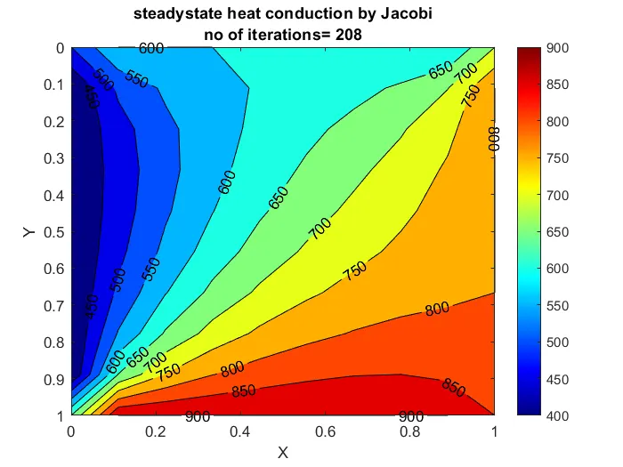
1. Jacobi method :
In the Jacobi method, we use the calculated value of the previous iteration in order to compute the current value.
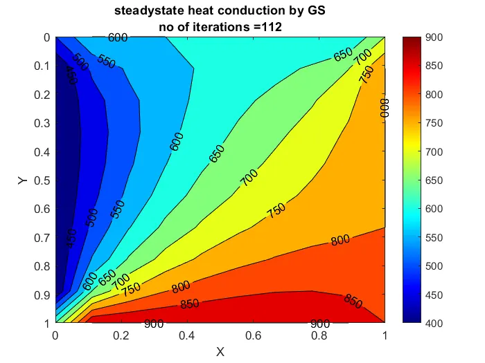
2. Gauss seidel method :
In the gauss seidel method, we use the latest updated value in order to compute the value in the current state.
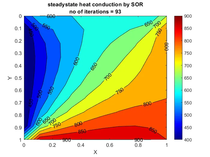
3. Successive over-relaxation(SOR):
This type of iterative solver is used to improve the convergence rate by including a factor called the relaxation factor.
MatLab code to solve 2D heat conduction using steady-state analysis:
Step1:clear all, close all, clc used to clear any previously defined values.
Step2:A suitable programme name is given.
Step3:Inputs are given
Step4:Boundary conditions are specified and corner temperatures are calculated.
Step5:Iterative solver is specified 1 for Jacobi(error=9e9; tol=1e-4 assumed)
(if, while and for loop are used)
`T(i,j)=(1/k)*((Told(i-1,j)+Told(i+1,j))/(dx^2))+(1/k)*((Told(i,j-1)+Told(i,j+1))/(dy^2))`
Step6:Iterative solver is specified 2 for Gauss seidel (error=9e9; tol=1e-4 assumed)
(if, while and for loop are used)
`T(i,j)=(1/k)*((T(i-1,j)+Told(i+1,j))/(dx^2))+(1/k)*((T(i,j-1)+Told(i,j+1))/(dy^2));`
and plot is done.
Step7:Iterative solver is specified 3 for SOR(error=9e9; tol=1e-4 assumed)
`omega=1.1 (taken)`
(if, while and for loop are used)
`T(i,j)=(1-omega)*Told(i,j)+omega*((1/k)*((T(i-1,j)+Told(i+1,j))/(dx^2))+(1/k)*((T(i,j-1)+Told(i,j+1))/(dy^2)));`
and plot is done.
Code:
clear all
close all
clc
% code to solve 2nd order 2D PDE steadystate
%d^2T/dx^2+d^2T/dy^2=0

%Inputs for 2nd order 2D PDE steadystate(nx=ny)
nx=10;
ny=10;
x=linspace(0,1,nx);
y=linspace(0,1,nx);
dx=x(2)-x(1);
dy=y(2)-y(1);
[xx,yy]=meshgrid(x,y);

%defining the boundary conditions
T=300*ones(nx,ny);

T_L = 400;
T_R = 800;
T_T = 600;
T_B = 900;

T(:,1) = T_L;
T(:,end) =T_R;
T(1,:)=T_T;
T(end,:)=T_B;


% defining the temperature at corner points
T(1,1) = (T_L+T_T)/2;
T(1,end) = (T_R+T_T)/2;
T(end,1) = (T_L+T_B)/2;
T(end,end) = (T_B+T_R)/2;
T_initial=T;
Told=T_initial;

iterativesolver=1;
error=9e9;
tol=1e-4;

%Jacobi Method

if iterativesolver==1
    jacobi_iter=1;
    while(error>tol)
       %space loop
        for i=2:nx-1
        for j=2:ny-1
            k=2*((dx^2+dy^2)/(dx^2*dy^2));
         T(i,j)=(1/k)*((Told(i-1,j)+Told(i+1,j))/(dx^2))+(1/k)*((Told(i,j-1)+Told(i,j+1))/(dy^2));

        end
        end
    error=max(max(abs(Told-T)));
    jacobi_iter=jacobi_iter+1;
    Told=T;
    end
    end


figure(1)
contourf(x,y,T,'ShowText','on');
colormap(jet);
colorbar;
set(gca,'YDIR','reverse')
xlabel('X')
ylabel('Y')
title_txt=sprintf('no of iterations= %d',jacobi_iter);
title( {'steadystate heat conduction by Jacobi';title_txt});
pause(0.03)


iterativesolver=2;
error=9e9;
tol=1e-4;
Told=T_initial;

%GS Method

if iterativesolver==2
  GS_iter=1;
   while(error>tol)
    %space loop
    for i=2:nx-1
    for j=2:ny-1
        k=2*((dx^2+dy^2)/(dx^2*dy^2));

     T(i,j)=(1/k)*((T(i-1,j)+Told(i+1,j))/(dx^2))+(1/k)*((T(i,j-1)+Told(i,j+1))/(dy^2));
    end
   end
   error=max(max(abs(Told-T)));
    GS_iter=GS_iter+1;
Told=T;
end
end


figure(2)
contourf(x,y,T,'ShowText','on');
colormap(jet);
colorbar;
set(gca,'YDIR','reverse')
xlabel('X')
ylabel('Y')
title_txt=sprintf('no of iterations =%d',GS_iter);
title( {'steadystate heat conduction by GS';title_txt});
pause(0.03)


iterativesolver=3;
error=9e9;
tol=1e-4;

%SOR Method
Told=T_initial;
if iterativesolver==3
SOR_iter=1;
 while(error>tol)
       %space loop
    for i=2:nx-1
    for j=2:ny-1
        k=2*((dx^2+dy^2)/(dx^2*dy^2));
   omega=1.1;

     T(i,j)=(1-omega)*Told(i,j)+omega*((1/k)*((T(i-1,j)+Told(i+1,j))/(dx^2))+(1/k)*((T(i,j-1)+Told(i,j+1))/(dy^2)));
    end
   end
   error=max(max(abs(Told-T)));
   SOR_iter=SOR_iter+1;
Told=T;
end
end


figure(3)
contourf(x,y,T,'ShowText','on');
colormap(jet);
colorbar;
set(gca,'YDIR','reverse')
xlabel('X')
ylabel('Y')
title_txt=sprintf('no of iterations = %d',SOR_iter);
title( {'steadystate heat conduction by SOR';title_txt});
pause(0.03)
For Transient heat conduction:
`(∂^2T)/(∂t^2)= alpha((∂^2T)/(∂x^2)+(∂^2T)/(∂y^2))`
Transient heat transfer can also be called unsteady-state heat transfer. This type of heat transfer only exists for a short duration of time. In transient heat transfers, the heat energy transferred through the medium is not constant. The heat flow rate keeps changing, and the cause of the varying rates of heat transfer can be either fluctuating temperature differences over the medium or changes in properties of the medium.
In the physical world, heat transfer starts as transient and then reaches a steady state until thermal equilibrium is reached.
MatLab code to solve 2D heat conduction using transient analysis:
1. Explicit
Step1:clear all, close all, clc used to clear any previously defined values.
Step2:A suitable program name is given. (explicit transient 2D heat conduction analysis is performed .)
Step3:Inputs are given
clear all
close all
clc

% code to solve 2nd order 2D PDE unsteadystate(or transient)(explicit)
%dT/dt=alpha*(d^2T/dx^2+d^2T/dy^2)

%Inputs for 2nd order 2D PDE(nx=ny)
nx=10;
ny=10;
dt=1e-3;

nt =1400;
x=linspace(0,1,nx);
y=linspace(0,1,nx);
dx=x(2)-x(1);
dy=y(2)-y(1);
[xx,yy]=meshgrid(x,y);


%defining the boundary conditions

T=300*ones(nx,ny);
T_L = 400;
T_R = 800;
T_T = 600;
T_B = 900;
Told=T;

T(:,1) = T_L;
T(:,end) =T_R;
T(1,:)=T_T;
T(end,:)=T_B;

% defining the temperature at corner points
T(1,1) = (T_L+T_T)/2;
T(1,end) = (T_R+T_T)/2;
T(end,1) = (T_L+T_B)/2;
T(end,end) = (T_B+T_R)/2;

tic
%time loop
for k = 1:nt
     error=1e-4;
%space loop
    for i=2:nx-1
        for j=2:ny-1
            alpha=2;
            k1=alpha*dt/(dx^2);
            k2=alpha*dt/(dy^2);

            T(i,j) = (Told(i,j) + k1*(Told(i+1,j) - 2*Told(i,j) + ...
                Told(i-1,j)) + k2*(Told(i,j+1) - 2*Told(i,j) + ...
                Told(i,j-1)));
        end
    end

% updating old values
Told = T;
end
time_taken = toc

figure(1)
contourf(x,y,T,'ShowText','on');
colormap(jet);
colorbar;
set(gca,'YDIR','reverse')
xlabel('X')
ylabel('Y')
title('2D heat conduction equation explicit transient');
2. Implicit(using Jacobi, Gauss seidel, and SOR iteration method)
Step1:clear all, close all, clc used to clear any previously defined values.
Step2:A suitable program name is given. (Implicit transient 2D heat conduction analysis is performed .)
Step3:Inputs are given
clear all
close all
clc

%2nd order 2D PDE unsteadystate(or transient)(implicit)

%Inputs for 2nd order 2D PDE(nx=ny)
nx=10;
ny=10;
dt=1e-3;

nt =1400;
x=linspace(0,1,nx);
y=linspace(0,1,nx);
dx=x(2)-x(1);
dy=y(2)-y(1);
[xx,yy]=meshgrid(x,y);


%defining the boundary conditions

T=300*ones(nx,ny);
T_L = 400;
T_R = 800;
T_T = 600;
T_B = 900;


T(:,1) = T_L;
T(:,end) =T_R;
T(1,:)=T_T;
T(end,:)=T_B;
T_initial=T;
Told=T_initial;

% defining the temperature at corner points
T(1,1) = (T_L+T_T)/2;
T(1,end) = (T_R+T_T)/2;
T(end,1) = (T_L+T_B)/2;
T(end,end) = (T_B+T_R)/2;


%2nd order 2D PDE unsteadystate(or transient)(implicit)

iterativesolver=1;
tol=1e-4;
Tprevious=Told;

%Jacobi Method

if iterativesolver==1
     tic
    jacobi_iter=1;
%time loop
     for k = 1:nt
         error=9e9;

%converging loop
        while(error>tol)
     %space loop
            for i=2:nx-1
                for j=2:ny-1
                    alpha=1.4;
                    k1=alpha*(dt/(dx^2));
                    k2=alpha*(dt/(dy^2));

                    term1=(1+(2*k1)+(2*k2))^-1;
                    term2= k1*term1;
                    term3= k2*term1;

                     H=Told(i-1,j)+Told(i+1,j);
                     V=Told(i,j-1)+Told(i,j+1);

                     T(i,j)= (term1*Tprevious(i,j))+(H*term2)+(V*term3);
                end
             end
            error=max(max(abs(Told-T)));
            Told=T;
            jacobi_iter=jacobi_iter+1;
        end
        t_error=max(max(abs(Told-T)));
        Tprevious=T;
     end
        time_taken = toc


figure(1)
contourf(x,y,T,'ShowText','on');
colormap(jet);
set(gca,'YDIR','reverse')
colorbar;
xlabel('X')
ylabel('Y')
title_txt=sprintf('no of iterations = %d',jacobi_iter);
title( {'unsteadystate heat conduction by jacobi';title_txt});
end


iterativesolver=2;
tol=1e-4;
T=T_initial;
Told=T_initial;
Tprevious=T_initial;


%GS Method

if iterativesolver==2
     tic
   GS_iter=1;
%time loop
     for k = 1:nt
         error=9e9;

%converging loop
     while(error>tol)
     %space loop
    for i=2:nx-1
    for j=2:ny-1

        alpha=1.4;
        k1=alpha*(dt/(dx^2));
        k2=alpha*(dt/(dy^2));

        term1=(1+(2*k1)+(2*k2))^-1;
        term2=k1*term1;
        term3=k2*term1;

        H=T(i-1,j)+Told(i+1,j);
        V=T(i,j-1)+Told(i,j+1);

     T(i,j)=(term1*Tprevious(i,j))+(H*term2)+(V*term3);
    end
    end
    error=max(max(abs(Told-T)));
    Told=T;
    GS_iter=GS_iter+1;
    end
    Tprevious=T;
    end
     time_taken = toc

figure(2)
contourf(x,y,T,'ShowText','on');
colormap(jet);
set(gca,'YDIR','reverse')
colorbar;
xlabel('X')
ylabel('Y')
title_txt=sprintf('no of iterations = %d',GS_iter);
title( {'unsteadystate heat conduction by GS';title_txt});
end

iterativesolver=3;
tol=1e-4;
T=T_initial;
Told=T_initial;
Tprevious=T_initial;

%SOR Method

if iterativesolver==3
     tic
 SOR_iter=1;
%time loop
     for k = 1:nt
          error=9e9;


%converging loop
     while(error>tol)
     %space loop
    for i=2:nx-1
    for j=2:ny-1

        alpha=1.4;
        omega=1.1;

        k1=alpha*(dt/(dx^2));
        k2=alpha*(dt/(dy^2));
        term1=(1+2*k1+2*k2)^-1;
        term2=k1*term1;
        term3=k2*term1;
        H=T(i-1,j)+Told(i+1,j);
        V=T(i,j-1)+Told(i,j+1);

     T(i,j)=(1-omega)*Told(i,j)+omega*(Tprevious(i,j)*term1+H*term2+V*term3);
    end
    end
    error=max(max(abs(Told-T)));
    Told=T;
     SOR_iter=SOR_iter+1;
     end
     Tprevious=T;
     end
     time_taken = toc

figure(3)
contourf(x,y,T,'ShowText','on');
colormap(jet);
set(gca,'YDIR','reverse')
colorbar;
xlabel('X')
ylabel('Y')
title_txt=sprintf('no of iterations = %d',SOR_iter);
title( {'unsteadystate heat conduction by SOR';title_txt});
end
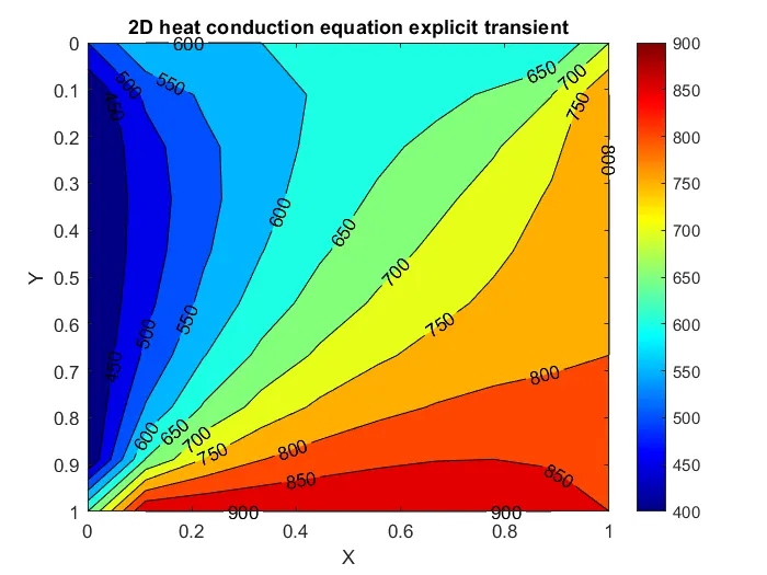
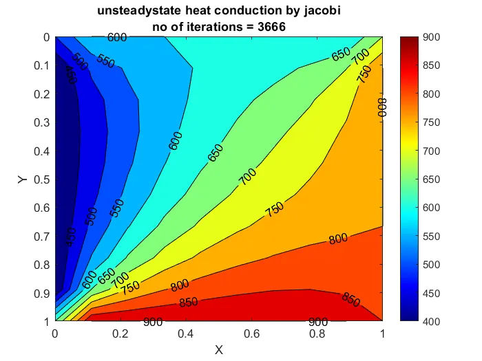
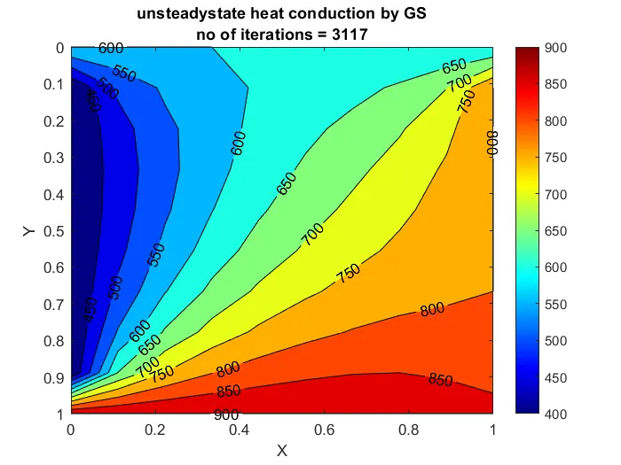
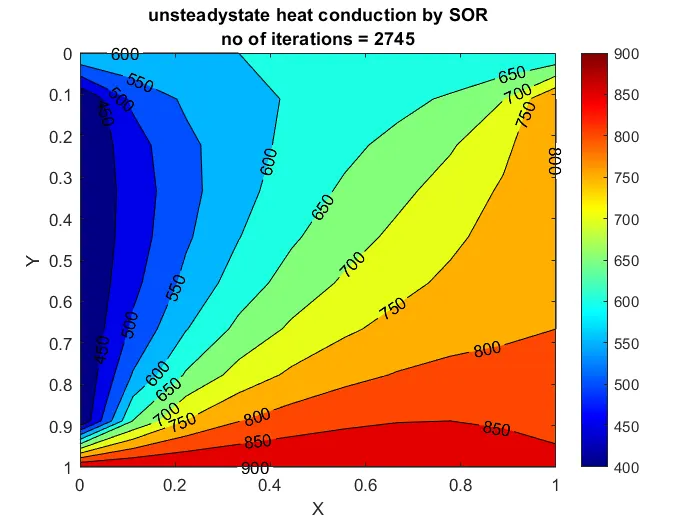
From the plotted graph, we can conclude the Successive Over-Relaxation method is more effective. The Number of Iteration and Simulation Runtime is very low compared to the other two methods Jacobi and Gauss Seidel. The Number of Iteration and Simulation Runtime is highest in Jacobi Method.
Jacobi>Gauss Seidel>SOR(No. of iteration)
CFL=K1+K2
CFL < 0.5 ,our solution is stable.