Week 5.1 - Mid term project - Solving the steady and unsteady 2D heat conduction problem
REPORT ON SOLVING A 2D HEAT CONDUCTION EQUATION USING THE POINT ITERATIVE TECHNIQUES
AIM
Solve the 2D heat conduction equation by using the point iterative techniques, using the following methods for solving implicit equations.
1. Jacobi
2. Gauss-seidel
3. Successive over-relaxation
Also to write code for both implicit and explicit schemes for transient analysis.
INPUT VALUES
The Boundary conditions for the problem are as follows;
Top Boundary = 600 K
Bottom Boundary = 900 K
Left Boundary = 400 K
Right Boundary = 800 K
Absolute error criteria is 1e-4
Number of nodes at x nx = 10
Number of nodes at y ny = 10
THEORY
The 2D convective heat conduction equation consists of two parts
1. Steady state
2. Unsteady/Transient state
The steady state equation is `(del^2T)/(delx^2)+(del^2T)/(dely^2) = 0`
and the unsteady state equation is `(delT)/(delt) = alpha((del^2T)/(delx^2)+(del^2T)/(dely^2))`
The equation which we use here to calculate the Temperature in the steady state condition is
`T_p^(n+1) = 1/k((T_L+T_R)/(Deltax^2)+(T_B+T_T)/(Deltay^2))^n`
where, T_L, T_B is the temperature at left and right side of the 2D equation and T_T and T_B are the top and bottom temperatures of the 2D equation.
where k = `(2(Deltax^2+Deltay^2))/(Deltax^2Deltay^2)`
This equation can to be calculated using 3 iteration techniques which helps to produce the required result in a lesser number of iterations and lesser time. In other words it is used to get a converged result at a faster rate.
1. Jacobi technique here we calculate T_p using the old temperature for all the temperature in the above equation i.e.
- In transient state we have two methods. Implicit and Explicit time integration, implicit time integration has n+1 terms on the RHS and usually while doing implicitily, we end up with matrix. We get a set of coupled linear equations. Whereas in explicit method we have n terms on the RHS and we get a set of uncoupled linear equations. It is also called as time marching method
- `T_p^(n+1) = T_p^n+alphaDeltat((T_R^n-2T_p^n+T_L^n)/(Deltax^2)+(T_T^n-2T_p^n+T_B^n)/(Deltay^2))`
- For implicit time integration the equation is `T_p^(n+1) = (T_p^n+k_1(T_L^(n+1)+T_R^(n+1))+k_2(T_T^(n+1)+T_B^(n+1)))/(1+2k_1+2k_2)`
- `k_1 = (alphaDeltat)/(Deltax^2)`, and `k_2 = (alphaDeltat)/(Deltay^2)`. Since it is implicit and we end up with matrix it is difficult to calculate 't' by solving the matrix, thus here we use the iterative solvers to solve the equation i.e here we use Jacobi, Gauss-siedel and Successive over relaxation techniques to solve the equation
BODY OF CONTENT
The program to solve the 2D equation under steady state condition:
clear all
close all
clc
%code to solve second order 2D pde
% d^2T/dx^2+d^2T/dy^2 = 0
%inputs
nx = 10;
ny = 10;
%initializing arrays and applying boundary conditions

x = linspace(0,1,nx);
y = linspace(0,1,ny);
dx = x(2)-x(1);
dy = y(2)-y(1);
%converting into 2D
[xx, yy] = meshgrid(x,y);
%initial guess value
t = 300*ones(nx,ny);
%BC
t(1,:) = 600;
t(end,:) = 900;
t(:,1) = 400;
t(:,end) = 800;
t(1,end) = 700;
t(1,1) = 500;
t(end,1) = 650;
t(end,end) = 850;
%initial condition
told =t;
t_initial = told;
iterative_solver = 2;
error = 1e-4;
tol = 1e-5;
k = (2*(dx^2+dy^2))/(dx^2*dy^2)
omega = 1.4;


%jacobi method

if iterative_solver == 1
    tic
   jacobi_iter = 1;
  while(error>tol)
    for i = 2:nx-1
     for j = 2:ny-1
         term1 = (told(i-1,j)+told(i+1,j))/(dx^2);
         term2 = (told(i,j-1)+told(i,j+1))/(dy^2);
      t(i,j) = (term1+term2)/k;
     end
    end

     error = max(max(abs(told-t)));
     told = t;
     jacobi_iter = jacobi_iter+1;
     time_taken = toc
     contourf(x,y,t)
     set(gca,'YDir','reverse')
    % plot(x,t,'LineWidth',3)
     xlabel('X ');
     ylabel('Y');
     %title_text = sprintf('iteration number = %d',jacobi_iter)
     text1 = sprintf('Number of Iteration = %d', jacobi_iter);
     text2 = sprintf('Simulation Time = %f', time_taken);
     title({'Steady State Heat Condustion profile by Jacobi'; text1; text2});

     %title(title_text)
     pause(0.03)
  end

end
%GS method

if iterative_solver == 2
    tic
   gs_iter = 1
  while(error>tol)
    for i = 2:nx-1
     for j = 2:ny-1
         term1 = (t(i-1,j)+told(i+1,j))/dx^2;
         term2 = (t(i,j-1)+told(i,j+1))/dy^2;
      t(i,j) = (term1+term2)/k;
     end
    end

     error = max(max(abs(told-t)));
     told = t;
     gs_iter = gs_iter+1;
     time_taken = toc
     contourf(x,y,t)
     set(gca,'YDir','reverse')
     %plot(X,Y,'LineWidth',3)
     xlabel('X')
     ylabel('Y')
     text1 = sprintf('Number of Iteration = %d', gs_iter);
     text2 = sprintf('Simulation Time = %f', time_taken);
     title({'Steady State Heat Condustion profile by Gauss-Siedel'; text1; text2});
%     title_text = sprintf('iteration number = %d',gs_iter)
%      title(title_text)

  end

end
%Successive over Relaxation
if iterative_solver == 3
   tic
   sor_iter = 1;
  while(error>tol)
    for i = 2:nx-1
     for j = 2:ny-1
         term1 = (t(i-1,j)+told(i+1,j))/(dx^2);
         term2 = (t(i,j-1)+told(i,j+1))/(dy^2);
      t(i,j) = ((told(i,j)*(1-omega))+(omega*((term1+term2))/k));
     end
    end

     error = max(max(abs(told-t)));
     told = t;
     sor_iter = sor_iter+1;
     time_taken = toc
     contourf(x,y,t)
     set(gca,'YDir','reverse')
     %plotting
     xlabel('X')
     ylabel('Y')
     text1 = sprintf('Number of Iteration = %d', sor_iter);
     text2 = sprintf('Simulation Time = %f', time_taken);
     title({'Steady State Heat Condustion profile by Successive over relaxation'; text1; text2});


  end

end
- In the above program first we input the input values i.e the number of nodes nx and ny as 10.
- Then we initialize the array and apply the boundary condititons by using linspace command. i.e the values of x and y are calculated using the linspace command and then we calculate the dx and dy
- Now we convert the 1D x and y into 2D using meshgrid command and then we guess the initial values using the ones command with nx rows and ny columns inside it and multiply it with 300, to create the initial temperature inside the boundary be 300.
- Then we input the given left, right, top and bottom boundary conditions. We also need to find the temperature at the 4 corners of the model. For that we take the average of adjecent points present to the corner points. i.e
- t(1,end) = 700, t(1,1) = 500, t(end,1) = 650, t(end,end) = 850; are the averages of the adjecent values of the corresponding pooints.(800+900)/2 = 850 like this other 3 corner points are calculated.
- Then the assumed t is stored as told and this told is then stored into a variable t_initial, which shows that at initial condition t =told = t_initial.
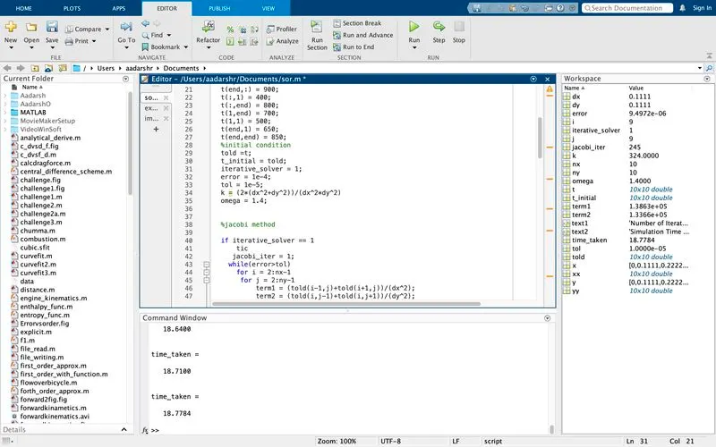
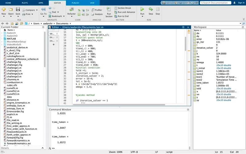
- Next step is to input the iterative solver number which helps the program to execute using the chosen method of iteration by the programmer. i.e if iterative_solver =1, jacobi technique is used, if it is 2 Gauss-Siedel method is used and if it is 3 SOR technique is used.
- Then we give the error condition and tolerance where error>tolerance and the program is required to execute till the given condition fails i.e when error<tolerance.
- Then the value of k and omega are given, where k is used in the steady state equation for Jacobi and GS method and omega is the scaling factor used in the equation of SOR technique.
- In the next step we use the Jacobi method of iteration to calculate `T_p^(n+1)`. For that first we create an if condition which checks whether the given iterative_solver =1,if it is 1 then the program is executed.
- Then the tic command is given to calculate the time taken to converge the equation and to calculate the number of iterations we initialise number 1 as the jacobi_iter.
- The next command is to execute the 2D equation inside the while condition i.e while(error>tolerance) i.e. until the above condition fails the program will be running inside the i and j loop which varies from 2:nx-1 and 2:ny-1. We give the limits from 2 upto nx-1 and ny-1 because we know the value of 't' at initial and final temperatures as they are the boundary conditions and inside these two loops the equation to calculate `T_p^(n+1)` which is denoted as t(i,j) is calculated i.e
term1 = (told(i-1,j)+told(i+1,j))/(dx^2);
term2 = (told(i,j-1)+told(i,j+1))/(dy^2);
t(i,j) = (term1+term2)/k;
- Here we divided the equation into two terms for easy understanding. And then we end the i and j loop for x and y using end command
- Now we calculate the absolute error which is the difference between told and the new t.For the next loop we should update the told which is the new t and then the iteration number is incremented a value of 1 after each loop. i.e jacobi_iter = jacobi_iter+1
- Then the time taken to complete the iteration is calculated using the toc command and displaying it by assigning it to a variable 'time_taken'.
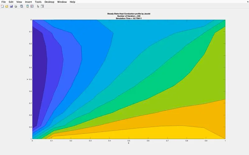
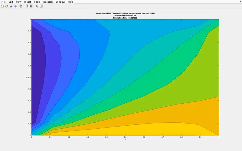
- Then we plot the x and y using the contourf command which creates a filled contour plot containing the isolines of matrix Z, where Z contains height values on the x-y plane. MATLAB automatically selects the contour lines to display. The column and row indices of Z are the x and y coordinates in the plane, respectively. Here x ,y and t are the coordinates
- Then we use a command called set(gca,'YDir','revrerse') which is used to reverse the values on the y axis from 1 to 0 rather than 0 to 1 from bottom to top.
- Then we plot label the x axis and y axis and provide the necessary title texts like displaying number of iterations and time taken to complete the same using the sprintf command and these texts are shown using title command.
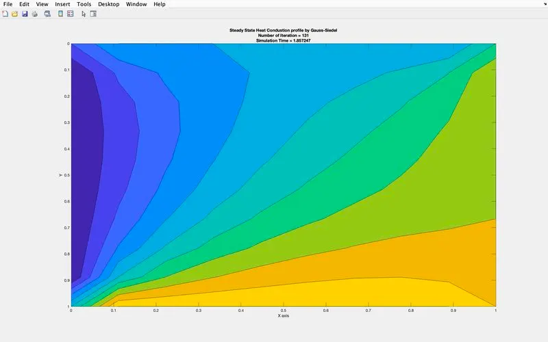
For Gauss-Siedel method the same procedure is followed only differences are in the if condition because to execute the GS technique the iterative number given by the programmer at the beginning should be 2 in place of 1 and the equation used to calculate has a small change as shown below, `T_p^(n+1)` which is denoted as t(i,j) is calculated as
term1 = (t(i-1,j)+told(i+1,j))/(dx^2);
term2 = (t(i,j-1)+told(i,j+1))/(dy^2);
t(i,j) = (term1+term2)/k;
Here t(i-1,j) is used inplace of told because in Gauss-Siedel method t is used in the equation which was calculated for the (n+1)th time step thus makes the equation converge at a much faster rate as compared to Jacobi method. We also change the variable to calculate the number of iterations as gs_iter which is assigned with an initial value of 1 and then incremented with a value of 1 after each cycle. The rest of the program is same as above
For Successive Over Relaxation technique where the general equation is `T_p^(n+1) = T_p^n(1-alpha)+alpha(T_(Jacobi) or T_(Gs))`
the equation and the if condition has the difference because to execute the SOR technique the iterative number given by the programmer at the beginning should be 3 in place of 1 and the equation used to calculate has a small change as shown below, `T_p^(n+1)` which is denoted as t(i,j) is calculated as
term1 = (t(i-1,j)+told(i+1,j))/(dx^2);
clear all
close all
clc
%code to solve second order 2D pde
% dT/dt = alpha*(d^2T/dx^2+d^2T/dy^2)
%inputs
nx = 10;
ny = 10;
alpha = 1.4;
%initializing arrays and applying boundary conditions

x = linspace(0,1,nx);
y = linspace(0,1,ny);
dx = x(2)-x(1);
dy = y(2)-y(1);
%time step
dt = 0.001;
%cfl value
k1 = (alpha*dt)/(dx^2);
k2 = (alpha*dt)/(dy^2);

%converting into 2D
[xx ,yy] = meshgrid(x,y);
%initial guess value
t = 300*ones(nx,ny);
%BC
t(1,:) = 600;
t(end,:) = 900;
t(:,1) = 400;
t(:,end) = 800;
t(1,end) = 700;
t(1) = 500;
t(end,1) = 650;
t(end,end) = 850;
%initial condition
told =t;
t_initial = told;
nt = 1400;
%transient at explicit condition

for m = 1:nt
    tic

  for i = 2:nx-1
      for j =2:ny-1
          term1 = k1*(told(i-1,j)-2*told(i,j)+told(i+1,j));
          term2 = k2 *(told(i,j-1)-2*told(i,j)+told(i,j+1));
          t(i,j) = told(i,j)+term1+term2;
      end
  end

     told = t;
end
time_taken = toc
   contourf(x,y,t)

    set(gca,'YDir','reverse')
     xlabel('X')
     ylabel('Y')
     text1 = sprintf('Simulation Time = %f', time_taken);
     title({'Transient state Explicit method'; text1});
In the above method we use the equation `(delT)/(delt) = alpha((del^2T)/(delx^2)+(del^2T)/(dely^2))`and the equation used to calculate the explicit time integration of unsteady condition is `T_p^(n+1) = T_p^n+alphaDeltat((T_R^n-2T_p^n+T_L^n)/(Deltax^2)+(T_T^n-2T_p^n+T_B^n)/(Deltay^2))`
This program is similar in format to that of steady state condition but still there are some differences in the input values and the equation used to calculate 't'
- In the above program first we input the input values i.e the number of nodes nx and ny as 10 and also input the value of constant alpha as 1.4
- Then we initialize the array and apply the boundary condititons by using linspace command. i.e the values of x and y are calculated using the linspace command and then we calculate the dx and dy
- Since it is a time marching equation we should input the value of dt which is given as 0.001
- Then the CFL values k1 and k2 are inputted.
- Now we convert the 1D x and y into 2D using meshgrid command and then we guess the initial values using the ones command with nx rows and ny columns inside it and multiply it with 300, to create the initial temperature inside the boundary be 300.
- Then we input the given left, right, top and bottom boundary conditions. We also need to find the temperature at the 4 corners of the model. For that we take the average of adjecent points present to the corner points.
- Then the assumed t is stored as told and this told is then stored into a variable t_initial, which shows that at initial condition t =told = t_initial.
- Now we give the number of time steps as 1400
- Then we create a time loop m which varies from 1 to nt and then the tic command is given to calculate the time taken
- Inside the i and j loop which varies from 2:nx-1 and 2:ny-1 which required for the 2D equation, the equation to calculate 't' is
- Here we divided the equation into two terms for easy understanding. And then we end the i and j loop for x and y using end command
- For the next loop we should update the told which is the new t. Then we end the time loop using end command
- Then the time taken to complete the iteration is calculated using the toc command and displaying it by assigning it to a variable 'time_taken'.
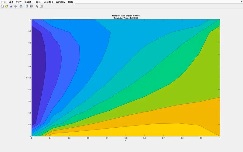
- Then we plot the x and y using the contourf command which creates a filled contour plot containing the isolines of matrix Z, where Z contains height values on the x-y plane
- Then we use a command called set(gca,'YDir','revrerse') which is used to reverse the values on the y axis from 1 to 0 rather than 0 to 1 from bottom to top.
- Then we plot label the x axis and y axis and provide the necessary title texts like displaying number of iterations and time taken to complete the same using the sprintf command and these texts are shown using title command.
The program to solve the 2D equation under unsteady/Transient state condition at Implicit time integration technique:
clear all
close all
clc
%code to solve second order 2D pde
% dT/dt = alpha*(d^2T/dx^2+d^2T/dy^2)
%inputs
nx = 10;
ny = 10;
%initializing arrays and applying boundary conditions

x = linspace(0,1,nx);
y = linspace(0,1,ny);
dx = x(2)-x(1);
dy = y(2)-y(1);
alpha = 1.4;
%converting into 2D
[xx ,yy] = meshgrid(x,y);
%initial guess value
t = 300*ones(nx,ny);
dt = 0.001;
%BC
t(1,:) = 600;
t(end,:) = 900;
t(:,1) = 400;
t(:,end) = 800;
t(1,end) = 700;
t(1,1) = 500;
t(end,1) = 650;
t(end,end) = 850;
%initial condition
told =t;
t_initial = told;
iterative_solver = 2;
tol = 1e-5;
k1 = (alpha*dt)/(dx^2);
k2 = (alpha*dt)/(dy^2);
nt = 1400;
omega = 1.4


%jacobi method

 if iterative_solver == 1
    tic;
   jacobi_iter = 1;
 for z = 1:nt
       error = 100;
  while(error>tol)
    for i = 2:nx-1
     for j = 2:ny-1
         term1 = (1+(2*(k1))+(2*(k2)))^(-1);
         term2 = k1*term1;
         term3 = k2*term1;
      t(i,j) = t_initial(i,j)*term1+term2*((told(i-1,j)+told(i+1,j)))+term3*((told(i,j-1)+told(i,j+1)));
     end
    end

     error = max(max(abs(told-t)));
     told = t;

     jacobi_iter = jacobi_iter+1;
  end
  t_initial = t;
 end
     time_taken = toc
     contourf(x,y,t)
     set(gca,'YDir','reverse')
    % plot(x,t,'LineWidth',3)
     xlabel('X')
     ylabel('Y')
     %title_text = sprintf('iteration number = %d',jacobi_iter)
     text1 = sprintf('Number of Iteration = %d', jacobi_iter);
     text2 = sprintf('Simulation Time = %f', time_taken);
     title({'Transient State Heat Condustion profile by Jacobi'; text1; text2});

     %title(title_text)
     pause(0.03)
  end

%GS method

if iterative_solver == 2
    tic
   gs_iter = 1;
 for z = 1:nt
       error = 100;
  while(error>tol)
    for i = 2:nx-1
     for j = 2:ny-1
         term1 = (1+(2*(k1))+(2*(k2)))^(-1);
         term2 = k1*term1;
         term3 = k2*term1;
      t(i,j) = t_initial(i,j)*term1+term2*((t(i-1,j)+told(i+1,j)))+term3*((t(i,j-1)+told(i,j+1)));
     end
    end

     error = max(max(abs(told-t)));
     told = t;
     gs_iter = gs_iter+1;
  end
  t_initial = t;
 end
     time_taken = toc
     contourf(x,y,t)
     set(gca,'YDir','reverse')
     %plot(X,Y,'LineWidth',3)
     xlabel('X')
     ylabel('Y')
     text1 = sprintf('Number of Iteration = %d', gs_iter);
     text2 = sprintf('Simulation Time = %f', time_taken);
     title({'Steady State Heat Condustion profile by Gauss-Siedel'; text1; text2});
     pause(0.03)

end
%Successive over Relaxation
 if iterative_solver == 3
   tic
   sor_iter = 1;
   for z = 1:nt
       error = 100;
   while(error>tol)
    for i = 2:nx-1
     for j = 2:ny-1
       term1 = (1+(2*(k1))+(2*(k2)))^(-1);
         term2 = k1*term1;
         term3 = k2*term1;
        t(i,j) = (t_initial(i,j)*(1-omega))+omega*((t_initial(i,j))*term1+term2*(t(i-1,j)+told(i+1,j))+term3*(t(i,j-1)+told(i,j+1)));
     end
    end

     error = max(max(abs(told-t)));
     told = t;
     sor_iter = sor_iter+1;
   end
        t_initial = t;
   end

     time_taken = toc
     contourf(x,y,t)
     set(gca,'YDir','reverse')
     %plot(x,t,'LineWidth',3)
     xlabel('X')
     ylabel('Y')
     text1 = sprintf('Number of Iteration = %d', sor_iter);
     text2 = sprintf('Simulation Time = %f', time_taken);
     title({'Steady State Heat Condustion profile by Successive over relaxation'; text1; text2});
     % title_text = sprintf('iteration number = %d',sor_iter)
     % title(title_text)


end
In implicit time integration, the equation has n+1 terms on the RHS and usually while doing implicitily, we end up with matrix. We get a set of coupled linear equations.
For implicit time integration the equation is `T_p^(n+1) = (T_p^n+k_1(T_L^(n+1)+T_R^(n+1))+k_2(T_T^(n+1)+T_B^(n+1)))/(1+2k_1+2k_2)`where`k_1 = (alphaDeltat)/(Deltax^2)`, and `k_2 = (alphaDeltat)/(Deltay^2)`. Here only the T_p^n value is known thus we use 'told' values and calculate the 't'. Since it is implicit and we end up with matrix it is difficult to calculate 't' by solving the matrix, thus here we use the iterative solvers to solve the equation i.e here we use Jacobi, Gauss-siedel and Successive over relaxation techniques to solve the equation.
- In the above program first we input the input values i.e the number of nodes nx and ny as 10 and also input the value of constant alpha as 1.4
- Then we initialize the array and apply the boundary condititons by using linspace command. i.e the values of x and y are calculated using the linspace command and then we calculate the dx and dy
- Since it is a time marching equation we should input the value of dt which is given as 0.001
- Then the CFL values k1 and k2 are inputted. In the CFL criteria (k1+k2) should be <= 0.5
- Now we convert the 1D x and y into 2D using meshgrid command and then we guess the initial values using the ones command with nx rows and ny columns inside it and multiply it with 300, to create the initial temperature inside the boundary be 300.
- Then we input the given left, right, top and bottom boundary conditions. We also need to find the temperature at the 4 corners of the model. For that we take the average of adjecent points present to the corner points.
- Next step is to input the iterative solver number which helps the program to execute using the chosen method of iteration by the programmer. i.e if iterative_solver =1, jacobi technique is used, if it is 2 Gauss-Siedel method is used and if it is 3 SOR technique is used.
- Then we give the tolerance and then the error inside the time loop ,where error>tolerance and the program is required to execute till the given condition fails i.e when error<tolerance.
- Here we give the tolerance value as 1e-5
- Then the assumed t is stored as told and this told is then stored into a variable t_initial, which shows that at initial condition t =told = t_initial.
- Now we give the number of time steps as 1400
- We also input scaling factor omega to solve using SOR method
- Now at first we use the Jacobi iteration technique, for that we use the if condition and check whether iterative_solver is 1 or not if it is 1 Jacobi technique is used for solving.
- Then the tic command is given to calculate the time taken and the number of iteration is initiated to be 1 and then we create a time loop z which varies from 1 to nt
- The while condition is given after that inside which the i loop and j loop is created.
- The next command is to execute the 2D equation inside the while condition i.e while(error>tolerance) i.e. until the above condition fails the program will be running inside the i and j loop which varies from 2:nx-1 and 2:ny-1. We give the limits from 2 upto nx-1 and ny-1 because we know the value of 't' at initial and final temperatures as they are the boundary conditions and inside these two loops the equation to calculate `T_p^(n+1)` which is denoted as t(i,j) is calculated i.e
term1 = (1+(2*(k1))+(2*(k2)))^(-1);term2 = k1*term1;term3 = k2*term1;t(i,j) = t_initial(i,j)*term1+term2*((told(i-1,j)+told(i+1,j)))+term3*((told(i,j-1)+told(i,j+1)));Here we divided the equation into three terms for easy understanding. And then we end the i and j loop for x and y using end command. The t_initial is a constant value for all the space loop and while loop and it is to be updated after each time loop
- Now we calculate the absolute error which is the difference between told and the new t.For the next loop we should update the told which is the new t and then the iteration number is incremented a value of 1 after each loop. i.e jacobi_iter = jacobi_iter+1
- Then 't_initial' is updated after the end command of while condition.
- Then the time taken to complete the iteration is calculated using the toc command and displaying it by assigning it to a variable 'time_taken'.
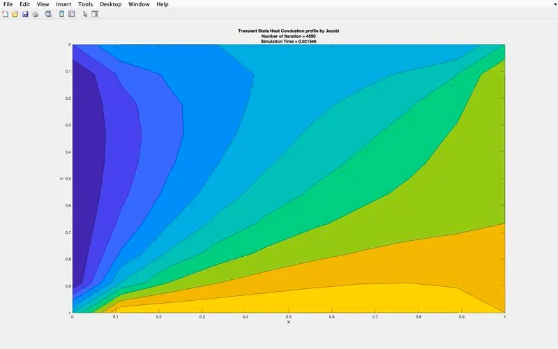
- Then we plot the x and y using the contourf command which creates a filled contour plot containing the isolines of matrix Z, where Z contains height values on the x-y plane
- Then we use a command called set(gca,'YDir','revrerse') which is used to reverse the values on the y axis from 1 to 0 rather than 0 to 1 from bottom to top.
- Then we plot label the x axis and y axis and provide the necessary title texts like displaying number of iterations and time taken to complete the same using the sprintf command and these texts are shown using title command.
For Gauss-Siedel iteration solver the same procedure is followed only differences are in the if condition because to execute the GS technique the iterative number given by the programmer at the beginning should be 2 in place of 1 and the equation used to calculate has a small change as shown below, `T_p^(n+1)` which is denoted as t(i,j) is calculated as
Here t(i-1,j) is used in place of told because in Gauss-Siedel method t is used in the equation which was calculated for the (n+1)th time step thus makes the equation converge at a much faster rate as compared to Jacobi method. We also change the variable to calculate the number of iterations as gs_iter which is assigned with an initial value of 1 and then incremented with a value of 1 after each cycle. The rest of the program is same as above, and also the iteration number is incremented a value of 1 after each loop. i.e gs_iter = gs_iter+1
For Successive Over Relaxation technique where the general equation is `T_p^(n+1) = T_p^n(1-alpha)+alpha(T_(Jacobi) or T_(Gs))`but here alpha is denoted as omega and
the equation and the if condition has the difference because to execute the SOR technique the iterative number given by the programmer at the beginning should be 3 in place of 1 and the equation used to calculate has a change as shown below, `T_p^(n+1)` which is denoted as t(i,j) is calculated as
clear all
close all
clc
%code to solve second order 2D pde
% d^2T/dx^2+d^2T/dy^2 = 0
%inputs
nx = 10;
ny = 10;
%initializing arrays and applying boundary conditions

x = linspace(0,1,nx);
y = linspace(0,1,ny);
dx = x(2)-x(1);
dy = y(2)-y(1);
%converting into 2D
[xx, yy] = meshgrid(x,y);
%initial guess value
t = 300*ones(nx,ny);
%BC
t(1,:) = 600;
t(end,:) = 900;
t(:,1) = 400;
t(:,end) = 800;
t(1,end) = 700;
t(1,1) = 500;
t(end,1) = 650;
t(end,end) = 850;
%initial condition
told =t;
t_initial = told;
iterative_solver = 1;
error = 1e-4;
tol = 1e-5;
k = (2*(dx^2+dy^2))/(dx^2*dy^2)
omega = 1.4;


%jacobi method

if iterative_solver == 1
    tic
   jacobi_iter = 1;
  while(error>tol)
    for i = 2:nx-1
     for j = 2:ny-1
         term1 = (told(i-1,j)+told(i+1,j))/(dx^2);
         term2 = (told(i,j-1)+told(i,j+1))/(dy^2);
      t(i,j) = (term1+term2)/k;
     end
    end

     error = max(max(abs(told-t)));
     told = t;
     jacobi_iter = jacobi_iter+1;
     time_taken = toc
     contourf(x,y,t)
     set(gca,'YDir','reverse')
    % plot(x,t,'LineWidth',3)
     xlabel('X ');
     ylabel('Y');
     %title_text = sprintf('iteration number = %d',jacobi_iter)
     text1 = sprintf('Number of Iteration = %d', jacobi_iter);
     text2 = sprintf('Simulation Time = %f', time_taken);
     title({'Steady State Heat Condustion profile by Jacobi'; text1; text2});

     %title(title_text)
     pause(0.03)
  end

end
%GS method

if iterative_solver == 2
    tic
   gs_iter = 1
  while(error>tol)
    for i = 2:nx-1
     for j = 2:ny-1
         term1 = (t(i-1,j)+told(i+1,j))/dx^2;
         term2 = (t(i,j-1)+told(i,j+1))/dy^2;
      t(i,j) = (term1+term2)/k;
     end
    end

     error = max(max(abs(told-t)));
     told = t;
     gs_iter = gs_iter+1;
     time_taken = toc
     contourf(x,y,t)
     set(gca,'YDir','reverse')
    %plotting
     xlabel('X')
     ylabel('Y')
     text1 = sprintf('Number of Iteration = %d', gs_iter);
     text2 = sprintf('Simulation Time = %f', time_taken);
     title({'Steady State Heat Condustion profile by Gauss-Siedel'; text1; text2});


  end

end
%Successive over Relaxation
if iterative_solver == 3
   tic
   sor_iter = 1;
  while(error>tol)
    for i = 2:nx-1
     for j = 2:ny-1
         term1 = (t(i-1,j)+told(i+1,j))/(dx^2);
         term2 = (t(i,j-1)+told(i,j+1))/(dy^2);
      t(i,j) = ((told(i,j)*(1-omega))+(omega*((term1+term2))/k));
     end
    end

     error = max(max(abs(told-t)));
     told = t;
     sor_iter = sor_iter+1;
     time_taken = toc
     contourf(x,y,t)
     set(gca,'YDir','reverse')
     %plot(x,t,'LineWidth',3)
     xlabel('X ')
     ylabel('Y')
     text1 = sprintf('Number of Iteration = %d', sor_iter);
     text2 = sprintf('Simulation Time = %f', time_taken);
     title({'Steady State Heat Condustion profile by Successive over relaxation'; text1; text2});
     % title_text = sprintf('iteration number = %d',sor_iter)
     % title(title_text)

  end

end
Using Gauss-Siedel technique:
clear all
close all
clc
%code to solve second order 2D pde
% d^2T/dx^2+d^2T/dy^2 = 0
%inputs
nx = 10;
ny = 10;
%initializing arrays and applying boundary conditions

x = linspace(0,1,nx);
y = linspace(0,1,ny);
dx = x(2)-x(1);
dy = y(2)-y(1);
%converting into 2D
[xx, yy] = meshgrid(x,y);
%initial guess value
t = 300*ones(nx,ny);
%BC
t(1,:) = 600;
t(end,:) = 900;
t(:,1) = 400;
t(:,end) = 800;
t(1,end) = 700;
t(1,1) = 500;
t(end,1) = 650;
t(end,end) = 850;
%initial condition
told =t;
t_initial = told;
iterative_solver = 2;
error = 1e-4;
tol = 1e-5;
k = (2*(dx^2+dy^2))/(dx^2*dy^2)
omega = 1.4;


%jacobi method

if iterative_solver == 1
    tic
   jacobi_iter = 1;
  while(error>tol)
    for i = 2:nx-1
     for j = 2:ny-1
         term1 = (told(i-1,j)+told(i+1,j))/(dx^2);
         term2 = (told(i,j-1)+told(i,j+1))/(dy^2);
      t(i,j) = (term1+term2)/k;
     end
    end

     error = max(max(abs(told-t)));
     told = t;
     jacobi_iter = jacobi_iter+1;
     time_taken = toc
     contourf(x,y,t)
     set(gca,'YDir','reverse')
    % plot(x,t,'LineWidth',3)
     xlabel('X ');
     ylabel('Y');
     %title_text = sprintf('iteration number = %d',jacobi_iter)
     text1 = sprintf('Number of Iteration = %d', jacobi_iter);
     text2 = sprintf('Simulation Time = %f', time_taken);
     title({'Steady State Heat Condustion profile by Jacobi'; text1; text2});

     %title(title_text)
     pause(0.03)
  end

end
%GS method

if iterative_solver == 2
    tic
   gs_iter = 1
  while(error>tol)
    for i = 2:nx-1
     for j = 2:ny-1
         term1 = (t(i-1,j)+told(i+1,j))/dx^2;
         term2 = (t(i,j-1)+told(i,j+1))/dy^2;
      t(i,j) = (term1+term2)/k;
     end
    end

     error = max(max(abs(told-t)));
     told = t;
     gs_iter = gs_iter+1;
     time_taken = toc
     contourf(x,y,t)
     set(gca,'YDir','reverse')
    %plotting
     xlabel('X axis')
     ylabel('Y')
     text1 = sprintf('Number of Iteration = %d', gs_iter);
     text2 = sprintf('Simulation Time = %f', time_taken);
     title({'Steady State Heat Condustion profile by Gauss-Siedel'; text1; text2});


  end

end
%Successive over Relaxation
if iterative_solver == 3
   tic
   sor_iter = 1;
  while(error>tol)
    for i = 2:nx-1
     for j = 2:ny-1
         term1 = (t(i-1,j)+told(i+1,j))/(dx^2);
         term2 = (t(i,j-1)+told(i,j+1))/(dy^2);
      t(i,j) = ((told(i,j)*(1-omega))+(omega*((term1+term2))/k));
     end
    end

     error = max(max(abs(told-t)));
     told = t;
     sor_iter = sor_iter+1;
     time_taken = toc
     contourf(x,y,t)
     set(gca,'YDir','reverse')
     %plot(x,t,'LineWidth',3)
     xlabel('X')
     ylabel('Y')
     text1 = sprintf('Number of Iteration = %d', sor_iter);
     text2 = sprintf('Simulation Time = %f', time_taken);
     title({'Steady State Heat Condustion profile by Successive over relaxation'; text1; text2});
     % title_text = sprintf('iteration number = %d',sor_iter)
     % title(title_text)

  end

end
Using Successive Over Relaxation technique:
clear all
close all
clc
%code to solve second order 2D pde
% d^2T/dx^2+d^2T/dy^2 = 0
%inputs
nx = 10;
ny = 10;
%initializing arrays and applying boundary conditions

x = linspace(0,1,nx);
y = linspace(0,1,ny);
dx = x(2)-x(1);
dy = y(2)-y(1);
%converting into 2D
[xx, yy] = meshgrid(x,y);
%initial guess value
t = 300*ones(nx,ny);
%BC
t(1,:) = 600;
t(end,:) = 900;
t(:,1) = 400;
t(:,end) = 800;
t(1,end) = 700;
t(1,1) = 500;
t(end,1) = 650;
t(end,end) = 850;
%initial condition
told =t;
t_initial = told;
iterative_solver = 3;
error = 1e-4;
tol = 1e-5;
k = (2*(dx^2+dy^2))/(dx^2*dy^2)
omega = 1.4;


%jacobi method

if iterative_solver == 1
    tic
   jacobi_iter = 1;
  while(error>tol)
    for i = 2:nx-1
     for j = 2:ny-1
         term1 = (told(i-1,j)+told(i+1,j))/(dx^2);
         term2 = (told(i,j-1)+told(i,j+1))/(dy^2);
      t(i,j) = (term1+term2)/k;
     end
    end

     error = max(max(abs(told-t)));
     told = t;
     jacobi_iter = jacobi_iter+1;
     time_taken = toc
     contourf(x,y,t)
     set(gca,'YDir','reverse')
    % plot(x,t,'LineWidth',3)
     xlabel('X ');
     ylabel('Y');
     %title_text = sprintf('iteration number = %d',jacobi_iter)
     text1 = sprintf('Number of Iteration = %d', jacobi_iter);
     text2 = sprintf('Simulation Time = %f', time_taken);
     title({'Steady State Heat Condustion profile by Jacobi'; text1; text2});

     %title(title_text)
     pause(0.03)
  end

end
%GS method

if iterative_solver == 2
    tic
   gs_iter = 1
  while(error>tol)
    for i = 2:nx-1
     for j = 2:ny-1
         term1 = (t(i-1,j)+told(i+1,j))/dx^2;
         term2 = (t(i,j-1)+told(i,j+1))/dy^2;
      t(i,j) = (term1+term2)/k;
     end
    end

     error = max(max(abs(told-t)));
     told = t;
     gs_iter = gs_iter+1;
     time_taken = toc
     contourf(x,y,t)
     set(gca,'YDir','reverse')
    %plotting
     xlabel('X axis')
     ylabel('Y')
     text1 = sprintf('Number of Iteration = %d', gs_iter);
     text2 = sprintf('Simulation Time = %f', time_taken);
     title({'Steady State Heat Condustion profile by Gauss-Siedel'; text1; text2});


  end

end
%Successive over Relaxation
if iterative_solver == 3
   tic
   sor_iter = 1;
  while(error>tol)
    for i = 2:nx-1
     for j = 2:ny-1
         term1 = (t(i-1,j)+told(i+1,j))/(dx^2);
         term2 = (t(i,j-1)+told(i,j+1))/(dy^2);
      t(i,j) = ((told(i,j)*(1-omega))+(omega*((term1+term2))/k));
     end
    end

     error = max(max(abs(told-t)));
     told = t;
     sor_iter = sor_iter+1;
     time_taken = toc
     contourf(x,y,t)
     set(gca,'YDir','reverse')
     %plot(x,t,'LineWidth',3)
     xlabel('X')
     ylabel('Y')
     text1 = sprintf('Number of Iteration = %d', sor_iter);
     text2 = sprintf('Simulation Time = %f', time_taken);
     title({'Steady State Heat Condustion profile by Successive over relaxation'; text1; text2});
     % title_text = sprintf('iteration number = %d',sor_iter)
     % title(title_text)

  end

end
The program to solve the 2D equation under unsteady/Transient state condition at Explicit time integration technique:
clear all
close all
clc
%code to solve second order 2D pde
% dT/dt = alpha*(d^2T/dx^2+d^2T/dy^2)
%inputs
nx = 10;
ny = 10;
alpha = 1.4;
%initializing arrays and applying boundary conditions

x = linspace(0,1,nx);
y = linspace(0,1,ny);
dx = x(2)-x(1);
dy = y(2)-y(1);
%time step
dt = 0.001;
%cfl value
k1 = (alpha*dt)/(dx^2);
k2 = (alpha*dt)/(dy^2);

%converting into 2D
[xx ,yy] = meshgrid(x,y);
%initial guess value
t = 300*ones(nx,ny);
%BC
t(1,:) = 600;
t(end,:) = 900;
t(:,1) = 400;
t(:,end) = 800;
t(1,end) = 700;
t(1) = 500;
t(end,1) = 650;
t(end,end) = 850;
%initial condition
told =t;
t_initial = told;
nt = 1400;
%transient at explicit condition

for m = 1:nt
    tic

  for i = 2:nx-1
      for j =2:ny-1
          term1 = k1*(told(i-1,j)-2*told(i,j)+told(i+1,j));
          term2 = k2 *(told(i,j-1)-2*told(i,j)+told(i,j+1));
          t(i,j) = told(i,j)+term1+term2;
      end
  end

     told = t;
end
time_taken = toc
   contourf(x,y,t)

    set(gca,'YDir','reverse')
     xlabel('X')
     ylabel('Y')
     text1 = sprintf('Simulation Time = %f', time_taken);
     title({'Transient state Explicit method'; text1});
The program to solve the 2D equation under unsteady/Transient state condition at Implicit time integration technique:
Using Jacobi technique:
clear all
close all
clc
%code to solve second order 2D pde
% dT/dt = alpha*(d^2T/dx^2+d^2T/dy^2)
%inputs
nx = 10;
ny = 10;
%initializing arrays and applying boundary conditions

x = linspace(0,1,nx);
y = linspace(0,1,ny);
dx = x(2)-x(1);
dy = y(2)-y(1);
alpha = 1.4;
%converting into 2D
[xx ,yy] = meshgrid(x,y);
%initial guess value
t = 300*ones(nx,ny);
dt = 0.001;
%BC
t(1,:) = 600;
t(end,:) = 900;
t(:,1) = 400;
t(:,end) = 800;
t(1,end) = 700;
t(1,1) = 500;
t(end,1) = 650;
t(end,end) = 850;
%initial condition
told =t;
t_initial = told;
iterative_solver = 1;
tol = 1e-5;
k1 = (alpha*dt)/(dx^2);
k2 = (alpha*dt)/(dy^2);
nt = 1400;
omega = 1.4


%jacobi method

 if iterative_solver == 1
    tic;
   jacobi_iter = 1;
 for z = 1:nt
       error = 100;
  while(error>tol)
    for i = 2:nx-1
     for j = 2:ny-1
         term1 = (1+(2*(k1))+(2*(k2)))^(-1);
         term2 = k1*term1;
         term3 = k2*term1;
      t(i,j) = t_initial(i,j)*term1+term2*((told(i-1,j)+told(i+1,j)))+term3*((told(i,j-1)+told(i,j+1)));
     end
    end

     error = max(max(abs(told-t)));
     told = t;

     jacobi_iter = jacobi_iter+1;
  end
  t_initial = t;
 end
     time_taken = toc
     contourf(x,y,t)
     set(gca,'YDir','reverse')
    % plot(x,t,'LineWidth',3)
     xlabel('X')
     ylabel('Y')
     %title_text = sprintf('iteration number = %d',jacobi_iter)
     text1 = sprintf('Number of Iteration = %d', jacobi_iter);
     text2 = sprintf('Simulation Time = %f', time_taken);
     title({'Transient State Heat Condustion profile by Jacobi'; text1; text2});

     %title(title_text)
     pause(0.03)
  end

%GS method

if iterative_solver == 2
    tic
   gs_iter = 1;
 for z = 1:nt
       error = 100;
  while(error>tol)
    for i = 2:nx-1
     for j = 2:ny-1
         term1 = (1+(2*(k1))+(2*(k2)))^(-1);
         term2 = k1*term1;
         term3 = k2*term1;
      t(i,j) = t_initial(i,j)*term1+term2*((t(i-1,j)+told(i+1,j)))+term3*((t(i,j-1)+told(i,j+1)));
     end
    end

     error = max(max(abs(told-t)));
     told = t;
     gs_iter = gs_iter+1;
  end
  t_initial = t;
 end
     time_taken = toc
     contourf(x,y,t)
     set(gca,'YDir','reverse')
     %plot(X,Y,'LineWidth',3)
     xlabel('X')
     ylabel('Y')
     text1 = sprintf('Number of Iteration = %d', gs_iter);
     text2 = sprintf('Simulation Time = %f', time_taken);
     title({'Steady State Heat Condustion profile by Gauss-Siedel'; text1; text2});
     pause(0.03)

end
%Successive over Relaxation
 if iterative_solver == 3
   tic
   sor_iter = 1;
   for z = 1:nt
       error = 100;
   while(error>tol)
    for i = 2:nx-1
     for j = 2:ny-1
       term1 = (1+(2*(k1))+(2*(k2)))^(-1);
         term2 = k1*term1;
         term3 = k2*term1;
        t(i,j) = (t_initial(i,j)*(1-omega))+omega*((t_initial(i,j))*term1+term2*(t(i-1,j)+told(i+1,j))+term3*(t(i,j-1)+told(i,j+1)));
     end
    end

     error = max(max(abs(told-t)));
     told = t;
     sor_iter = sor_iter+1;
   end
        t_initial = t;
   end

     time_taken = toc
     contourf(x,y,t)
     set(gca,'YDir','reverse')
     %plot(x,t,'LineWidth',3)
     xlabel('X')
     ylabel('Y')
     text1 = sprintf('Number of Iteration = %d', sor_iter);
     text2 = sprintf('Simulation Time = %f', time_taken);
     title({'Steady State Heat Condustion profile by Successive over relaxation'; text1; text2});
     % title_text = sprintf('iteration number = %d',sor_iter)
     % title(title_text)


end
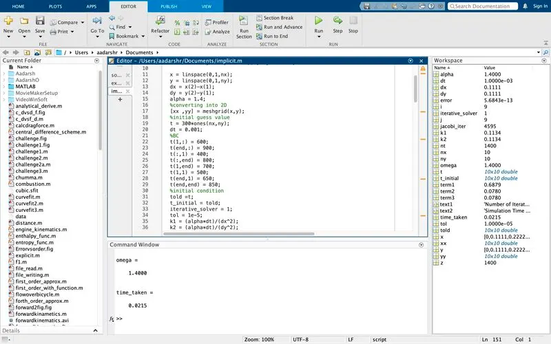
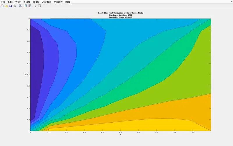
Using Gauss-Siedel technique:
clear all
close all
clc
%code to solve second order 2D pde
% dT/dt = alpha*(d^2T/dx^2+d^2T/dy^2)
%inputs
nx = 10;
ny = 10;
%initializing arrays and applying boundary conditions

x = linspace(0,1,nx);
y = linspace(0,1,ny);
dx = x(2)-x(1);
dy = y(2)-y(1);
alpha = 1.4;
%converting into 2D
[xx ,yy] = meshgrid(x,y);
%initial guess value
t = 300*ones(nx,ny);
dt = 0.001;
%BC
t(1,:) = 600;
t(end,:) = 900;
t(:,1) = 400;
t(:,end) = 800;
t(1,end) = 700;
t(1,1) = 500;
t(end,1) = 650;
t(end,end) = 850;
%initial condition
told =t;
t_initial = told;
iterative_solver = 2;
tol = 1e-5;
k1 = (alpha*dt)/(dx^2);
k2 = (alpha*dt)/(dy^2);
nt = 1400;
omega = 1.4


%jacobi method

 if iterative_solver == 1
    tic;
   jacobi_iter = 1;
 for z = 1:nt
       error = 100;
  while(error>tol)
    for i = 2:nx-1
     for j = 2:ny-1
         term1 = (1+(2*(k1))+(2*(k2)))^(-1);
         term2 = k1*term1;
         term3 = k2*term1;
      t(i,j) = t_initial(i,j)*term1+term2*((told(i-1,j)+told(i+1,j)))+term3*((told(i,j-1)+told(i,j+1)));
     end
    end

     error = max(max(abs(told-t)));
     told = t;

     jacobi_iter = jacobi_iter+1;
  end
  t_initial = t;
 end
     time_taken = toc
     contourf(x,y,t)
     set(gca,'YDir','reverse')
    % plot(x,t,'LineWidth',3)
     xlabel('X')
     ylabel('Y')
     %title_text = sprintf('iteration number = %d',jacobi_iter)
     text1 = sprintf('Number of Iteration = %d', jacobi_iter);
     text2 = sprintf('Simulation Time = %f', time_taken);
     title({'Transient State Heat Condustion profile by Jacobi'; text1; text2});

     %title(title_text)
     pause(0.03)
  end

%GS method

if iterative_solver == 2
    tic
   gs_iter = 1;
 for z = 1:nt
       error = 100;
  while(error>tol)
    for i = 2:nx-1
     for j = 2:ny-1
         term1 = (1+(2*(k1))+(2*(k2)))^(-1);
         term2 = k1*term1;
         term3 = k2*term1;
      t(i,j) = t_initial(i,j)*term1+term2*((t(i-1,j)+told(i+1,j)))+term3*((t(i,j-1)+told(i,j+1)));
     end
    end

     error = max(max(abs(told-t)));
     told = t;
     gs_iter = gs_iter+1;
  end
  t_initial = t;
 end
     time_taken = toc
     contourf(x,y,t)
     set(gca,'YDir','reverse')
     %plot(X,Y,'LineWidth',3)
     xlabel('X')
     ylabel('Y')
     text1 = sprintf('Number of Iteration = %d', gs_iter);
     text2 = sprintf('Simulation Time = %f', time_taken);
     title({'Steady State Heat Condustion profile by Gauss-Siedel'; text1; text2});
     pause(0.03)

end
%Successive over Relaxation
 if iterative_solver == 3
   tic
   sor_iter = 1;
   for z = 1:nt
       error = 100;
   while(error>tol)
    for i = 2:nx-1
     for j = 2:ny-1
       term1 = (1+(2*(k1))+(2*(k2)))^(-1);
         term2 = k1*term1;
         term3 = k2*term1;
        t(i,j) = (t_initial(i,j)*(1-omega))+omega*((t_initial(i,j))*term1+term2*(t(i-1,j)+told(i+1,j))+term3*(t(i,j-1)+told(i,j+1)));
     end
    end

     error = max(max(abs(told-t)));
     told = t;
     sor_iter = sor_iter+1;
   end
        t_initial = t;
   end

     time_taken = toc
     contourf(x,y,t)
     set(gca,'YDir','reverse')
     %plot(x,t,'LineWidth',3)
     xlabel('X')
     ylabel('Y')
     text1 = sprintf('Number of Iteration = %d', sor_iter);
     text2 = sprintf('Simulation Time = %f', time_taken);
     title({'Steady State Heat Condustion profile by Successive over relaxation'; text1; text2});
     % title_text = sprintf('iteration number = %d',sor_iter)
     % title(title_text)


end
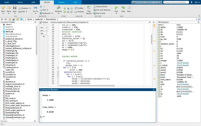
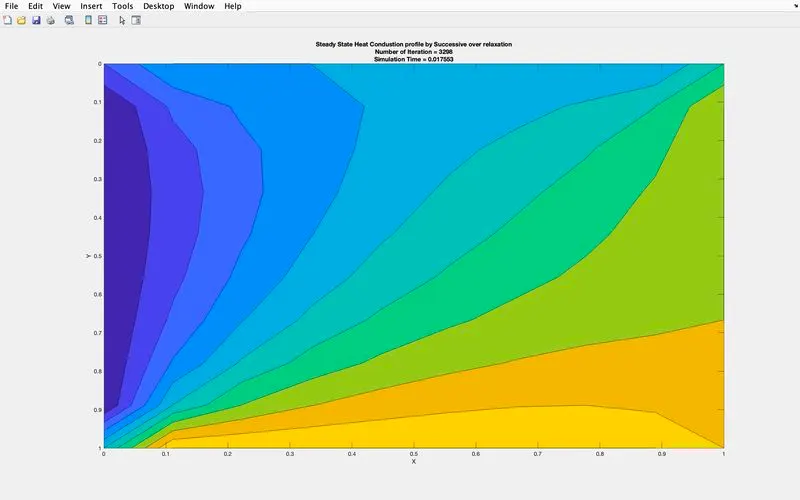
Using Successive Over Relaxation technique:
clear all
close all
clc
%code to solve second order 2D pde
% dT/dt = alpha*(d^2T/dx^2+d^2T/dy^2)
%inputs
nx = 10;
ny = 10;
%initializing arrays and applying boundary conditions

x = linspace(0,1,nx);
y = linspace(0,1,ny);
dx = x(2)-x(1);
dy = y(2)-y(1);
alpha = 1.4;
%converting into 2D
[xx ,yy] = meshgrid(x,y);
%initial guess value
t = 300*ones(nx,ny);
dt = 0.001;
%BC
t(1,:) = 600;
t(end,:) = 900;
t(:,1) = 400;
t(:,end) = 800;
t(1,end) = 700;
t(1,1) = 500;
t(end,1) = 650;
t(end,end) = 850;
%initial condition
told =t;
t_initial = told;
iterative_solver = 3;
tol = 1e-5;
k1 = (alpha*dt)/(dx^2);
k2 = (alpha*dt)/(dy^2);
nt = 1400;
omega = 1.4


%jacobi method

 if iterative_solver == 1
    tic;
   jacobi_iter = 1;
 for z = 1:nt
       error = 100;
  while(error>tol)
    for i = 2:nx-1
     for j = 2:ny-1
         term1 = (1+(2*(k1))+(2*(k2)))^(-1);
         term2 = k1*term1;
         term3 = k2*term1;
      t(i,j) = t_initial(i,j)*term1+term2*((told(i-1,j)+told(i+1,j)))+term3*((told(i,j-1)+told(i,j+1)));
     end
    end

     error = max(max(abs(told-t)));
     told = t;

     jacobi_iter = jacobi_iter+1;
  end
  t_initial = t;
 end
     time_taken = toc
     contourf(x,y,t)
     set(gca,'YDir','reverse')
    % plot(x,t,'LineWidth',3)
     xlabel('X')
     ylabel('Y')
     %title_text = sprintf('iteration number = %d',jacobi_iter)
     text1 = sprintf('Number of Iteration = %d', jacobi_iter);
     text2 = sprintf('Simulation Time = %f', time_taken);
     title({'Transient State Heat Condustion profile by Jacobi'; text1; text2});

     %title(title_text)
     pause(0.03)
  end

%GS method

if iterative_solver == 2
    tic
   gs_iter = 1;
 for z = 1:nt
       error = 100;
  while(error>tol)
    for i = 2:nx-1
     for j = 2:ny-1
         term1 = (1+(2*(k1))+(2*(k2)))^(-1);
         term2 = k1*term1;
         term3 = k2*term1;
      t(i,j) = t_initial(i,j)*term1+term2*((t(i-1,j)+told(i+1,j)))+term3*((t(i,j-1)+told(i,j+1)));
     end
    end

     error = max(max(abs(told-t)));
     told = t;
     gs_iter = gs_iter+1;
  end
  t_initial = t;
 end
     time_taken = toc
     contourf(x,y,t)
     set(gca,'YDir','reverse')
     %plot(X,Y,'LineWidth',3)
     xlabel('X')
     ylabel('Y')
     text1 = sprintf('Number of Iteration = %d', gs_iter);
     text2 = sprintf('Simulation Time = %f', time_taken);
     title({'Steady State Heat Condustion profile by Gauss-Siedel'; text1; text2});
     pause(0.03)

end
%Successive over Relaxation
 if iterative_solver == 3
   tic
   sor_iter = 1;
   for z = 1:nt
       error = 100;
   while(error>tol)
    for i = 2:nx-1
     for j = 2:ny-1
       term1 = (1+(2*(k1))+(2*(k2)))^(-1);
         term2 = k1*term1;
         term3 = k2*term1;
        t(i,j) = (t_initial(i,j)*(1-omega))+omega*((t_initial(i,j))*term1+term2*(t(i-1,j)+told(i+1,j))+term3*(t(i,j-1)+told(i,j+1)));
     end
    end

     error = max(max(abs(told-t)));
     told = t;
     sor_iter = sor_iter+1;
   end
        t_initial = t;
   end

     time_taken = toc
     contourf(x,y,t)
     set(gca,'YDir','reverse')
     %plot(x,t,'LineWidth',3)
     xlabel('X')
     ylabel('Y')
     text1 = sprintf('Number of Iteration = %d', sor_iter);
     text2 = sprintf('Simulation Time = %f', time_taken);
     title({'Steady State Heat Condustion profile by Successive over relaxation'; text1; text2});
     % title_text = sprintf('iteration number = %d',sor_iter)
     % title(title_text)


end
RESULT
The program to solve the 2D heat conduction equation by using the point iterative techniques, using the following methods for solving implicit equations
1. Jacobi
2. Gauss-seidel
3. Successive over-relaxation
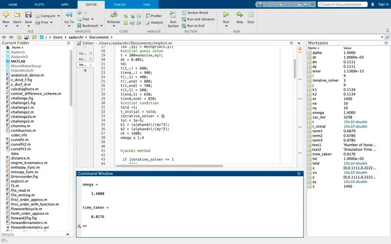
Also to write code for both implicit and explicit schemes for transient analysis is successfully completed and the following result is obtained i.e `(Number of iterations)_(Jacobi)>(Number of iterations)_(GS)>(Number of iterations)_(SOR)`i.e SOR solves the equation at lesser number of iterations and lesser time than the other two. Which resembles that SOR technique is the most suitable one of the three for the 2D heat conduction equation