Week 5.1 - Mid term project - Solving the steady and unsteady 2D heat conduction problem
Aim:
To Solve the 2D heat conduction equation by using the point iterative techniques that were taught in the class. The Boundary conditions for the problem are as follows given below.
Objective:
Top Boundary = 600 K
Bottom Boundary = 900 K
Left Boundary = 400 K
Right Boundary = 800 K
You will implement the following methods for solving implicit equations.
- Jacobi
- Gauss-seidel
- Successive over-relaxation
Your absolute error criteria is 1e-4
Above all are the challenge given instruction we should follow these steps. And solve this challenge.
Theory:
There are two types of heat conductions first one is transient and second one is steady state heat conduction.
Transient heat conduction A state of heat conduction in which the temperature of the body is unsteady in nature. The time temperature at any given point in a body will vary with time thus either increasing or decreasing in the process but not staying the same with respect to time.
Steady state heat conduction:
Steady state conduction is the form of conduction that happens when the temperature difference driving the conduction are constant so that the spatial distribution of temperatures in the conduction object does not change any further.
Boundary condition:
DISCRETIZATION:
The heat conduction equation is a PDE and must be discretized so as to solve it.
STEADY STATE:
`(∂^2 T)/(∂x^2 )+(∂^2 T)/(∂y^2 )=0`
Discretization method,
`T_P=1/k ((T_L+T_R)/(dx^2 ))+((T_T+T_B)/(dy^2 ))`
For solving the equation implicitly using:
Jacobi Iteration and Gauss-Seidel Iteration, the equation can be written as
`T(i,j)=1/k ((T_((i-1,j) )+T_old(i+1,j) )/(dx^2 ))+1/k ((T_((i,j-1) )+T_old(i,j+1) )/(dy^2 ))`
Successive over Relaxation Iteration, the equation can be written as
`T(i,j)=(1-ω)*T_old(i,j) +ω*[1/k ((T_((i-1,j) )+T_old(i+1,j) )/(dx^2 ))+1/k ((T_((i,j-1) )+T_old(i,j+1) )/(dy^2 ))]`
If ω >1, over relaxation
`ω<1 under relaxation
TRANSIENT STATE:
`(∂^2 T)/(∂t^2 )=∝((∂^2 T)/(∂x^2 )+(∂^2 T)/(∂y^2 ))`
Discretization method,
`T_(P^(n+1) )=T_(P^n )+∝*dt[((T_L-2T_P+T_R)/(dx^2 ))+((T_T-2T_P+T_B)/(dy^2 ))]`
To solve this explicitly, no iterative techniques are needed, since all the values are known. Hence,
`T_(P^(n+1) )=T_(P^n )+k1*(T(i-1,j)-2T(i,j)+T(i+1,j)+k2*(T(i,j-1)-2T(i,j)+T(i,j-1))`
For solving the equation implicitly rearranging method,
`T_(P^(n+1) )=1/(1+2k1+2k2)[T_(P^n )+k1*(〖T_L+T_R)〗^(n+1)+k2*(T_T+T_B )^(n+1)]`
Steady state heat conduction implicit code`
clear all
close all
clc

% inputs
nx=10;
ny=nx;
x=linspace(0,1,nx);
y=linspace(0,1,ny);
dx=x(2)-x(1);
dy=y(2)-y(1);

T_l=400;
T_r=800;
T_t=600;
T_b=900;
T_in=300; %value of T in all other points except the boundaries
T=T_in*ones(10,1)*ones(1,10); %creating a square grid of temperature

%Introducing the boundary conditions except the corners
T(2:ny-1,1)=T_l;
T(2:ny-1,ny)=T_r;
T(1,2:nx-1)=T_t;
T(ny,2:nx-1)=T_b;

%computing corner values
T(1,1)=(T_t+T_l)/2;
T(10,1)=(T_b+T_l)/2;
T(1,10)=(T_t+T_r)/2;
T(10,10)=(T_b+T_r)/2;
error=9e9;
tol=1e-4;
k=2*(dx^2+dy^2)/(dx^2*dy^2);
Told=T;
iteration_number=3; %can be changed to access different methods

%JACOBI ITERATION
if iteration_number==1
jacobi=1;
while(error>tol)
for i=2:nx-1
for j=2:ny-1
term1=(Told(i-1,j)+Told(i+1,j))/(k*dx^2);
term2=(Told(i,j-1)+Told(i,j+1))/(k*dy^2);
T(i,j)=term1+term2;
end
end
error=max(max(abs(Told-T)));
Told=T;
jacobi=jacobi+1;
contourf(x,y,T,'ShowText','on')
set(gca,'YDIR','reverse')
c=colorbar;
c.Label.String='Temperature (K)';
title_text=sprintf('no: of jacobi iterations=%d',jacobi);
title(title_text);
pause(0.03);
end
end

%GAUSS SIEDEL ITERATION
if iteration_number==2
gauss=1;
while(error>tol)
for i=2:nx-1
for j=2:nx-1
term1=(T(i-1,j)+Told(i+1,j))/(k*dx^2);
term2=(T(i,j-1)+Told(i,j+1))/(k*dx^2);
T(i,j)=term1+term2;
end
end
error=max(max(abs(Told-T)));
Told=T;
gauss=gauss+1;
contourf(x,y,T,'ShowText','on')
set(gca,'YDIR','reverse')
c=colorbar;
c.Label.String='Temperature (K)';
title_text=sprintf('no: of gauss iterations=%d',gauss);
title(title_text);
pause(0.03);
end
end

%SUCCESSIVE OVER RELAXATION
omega=1.2; %relaxation factor

if iteration_number==3
SOR=1;
while(error>tol)
for i=2:nx-1
for j=2:nx-1
term1=(T(i-1,j)+Told(i+1,j))/(k*dx^2);
term2=(T(i,j-1)+Told(i,j+1))/(k*dx^2);
T(i,j)=(1-omega)*Told(i,j)+omega*(term1+term2);
end
end

error=max(max(abs(Told-T)));
Told=T;
SOR=SOR+1;
contourf(x,y,T,'ShowText','on')
set(gca,'YDIR','reverse')
c=colorbar;
c.Label.String='Temperature (K)';
title_text=sprintf('no: of sor iterations=%d',SOR);
title(title_text);
pause(0.03);
end
end
Transient heat conduction explicit code:
clear all
close all
clc

% inputs
nx=10;
ny=nx;
x=linspace(0,1,nx);
y=linspace(0,1,ny);
dx=x(2)-x(1);
dy=y(2)-y(1);

T_l=400;
T_r=800;
T_t=600;
T_b=900;
T_in=300; %value of T in all other points except the boundaries
T=T_in*ones(10,1)*ones(1,10); %creating a square grid of temperature

%Introducing the boundary conditions except the corners
T(2:ny-1,1)=T_l;
T(2:ny-1,ny)=T_r;
T(1,2:nx-1)=T_t;
T(ny,2:nx-1)=T_b;

%computing corner values
T(1,1)=(T_t+T_l)/2;
T(10,1)=(T_b+T_l)/2;
T(1,10)=(T_t+T_r)/2;
T(10,10)=(T_b+T_r)/2;
Told=T;
dt=1e-3;
alpha=1.4;
k1=alpha*dt/dx^2;
k2=k1;
CFL=k1+k2;
error=1;
tol=1e-4;
iteration=1;

while(error>tol)
for i=2:nx-1
for j=2:ny-1
term1=Told(i-1,j)-2*Told(i,j)+Told(i+1,j);
term2=Told(i,j-1)-2*Told(i,j)+Told(i,j+1);
T(i,j)=Told(i,j)+k1*term1+k2*term2 ;
end
end

error=max(max(abs(T-Told)));
Told=T;
iteration=iteration+1;
contourf(x,y,T,'ShowText','on')
set(gca,'YDIR','reverse')
c=colorbar;
c.Label.String='Temperature (K)';
title_text=sprintf('no: of iterations=%d',iteration);
title(title_text);
pause(0.03);
end
Transient heat conduction implicit code:
clear all
close all
clc

%inputs
nx=10;
ny=nx;

%creating x and y grids
x=linspace(0,1,nx);
y=linspace(0,1,ny);
dx=x(2)-x(1);
dy=y(2)-y(1);

%boundary conditions
T_l=400;
T_r=800;
T_t=600;
T_b=900;
T_in=300; %value of T in all other points except the boundaries
T=T_in*ones(10,1)*ones(1,10); %creating a square grid of temperature

%Introducing the boundary conditions except the corners
T(2:ny-1,1)=T_l;
T(2:ny-1,ny)=T_r;
T(1,2:nx-1)=T_t;
T(ny,2:nx-1)=T_b;

%computing corner values
T(1,1)=(T_t+T_l)/2;
T(10,1)=(T_b+T_l)/2;
T(1,10)=(T_t+T_r)/2;
T(10,10)=(T_b+T_r)/2;
alpha=1.4; %thermal diffusion
omega=1.2; %relaxation factor
dt=1e-3;
nt=1400;
k1=alpha*dt/dx^2;
k2=k1;
CFL=k1+k2;
error=9e9;
t_error=9e9;
tol=1e-4;
jacobi_implicit=1;
gauss_implicit=1;
SOR_implicit=1;
Told=T; %for the old iteration
Tprev=T; %for the old time step
Tinitial=T;

%JACOBI
while(t_error>tol)
error=9e9;
while(error>tol)
for i=2:nx-1
for j=2:ny-1
term1=(1+2*k1+2*k2)^-1;
term2=k1*term1;
term3=k2*term1;
H=Told(i-1,j)+Told(i+1,j);
V=Told(i,j-1)+Told(i,j+1);
T(i,j)=(Tprev(i,j)*term1)+H*term2+V*term3;
end
end
error=max(max(abs(Told-T)));
Told=T;
jacobi_implicit=jacobi_implicit+1;
end
t_error = max(max(abs(Tprev-T)));
Tprev=T;
end

figure(1)
contourf(x,y,T,'ShowText','on')
set(gca,'YDIR','reverse')
c=colorbar;
c.Label.String='Temperature (K)';
title_text=sprintf('no: of jacobi iterations=%d',jacobi_implicit);
title(title_text);
pause(0.03);

%GAUSS
T = Tinitial;
Told = Tinitial;
Tprev = Tinitial;
t_error=9e9;
while(t_error>tol)
error=9e9;
while(error>tol)
for i=2:nx-1
for j=2:ny-1
term1=(1+2*k1+2*k2)^-1;
term2=k1*term1;
term3=k2*term1;
H=T(i-1,j)+Told(i+1,j);
V=T(i,j-1)+Told(i,j+1);
T(i,j)=(Tprev(i,j)*term1)+H*term2+V*term3;
end
end
error=max(max(abs(Told-T)));
Told=T;
gauss_implicit=gauss_implicit+1;
end
t_error = max(max(abs(Tprev-T)));
Tprev=T;
end
figure(2)
contourf(x,y,T,'ShowText','on')
set(gca,'YDIR','reverse')
c=colorbar;
c.Label.String='Temperature (K)';
title_text=sprintf('no: of gauss iterations=%d',gauss_implicit);
title(title_text);
pause(0.03);

%SOR
T = Tinitial;
Told = Tinitial;
Tprev = Tinitial;
t_error=9e9;

while(t_error>tol)
error=9e9;
while(error>tol)
for i=2:nx-1
for j=2:ny-1
term1=(1+2*k1+2*k2)^-1;
term2=k1*term1;
term3=k2*term1;
H=T(i-1,j)+Told(i+1,j);
V=T(i,j-1)+Told(i,j+1);
T(i,j)=(1-omega)*Told(i,j)+omega*(Tprev(i,j)*term1+H*term2+V*term3);
end
end
error=max(max(abs(Told-T)));
Told=T;
SOR_implicit=SOR_implicit+1;
end
t_error = max(max(abs(Tprev-T)));
Tprev=T;
end
figure(3)
contourf(x,y,T,'ShowText','on')
set(gca,'YDIR','reverse')
c=colorbar;
c.Label.String='Temperature (K)';
title_text=sprintf('no: of SOR iterations=%d',SOR_implicit);
title(title_text);
pause(0.03);
Results:
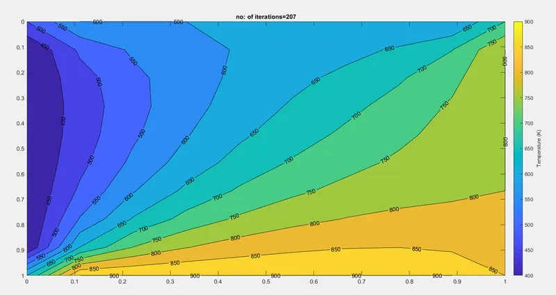
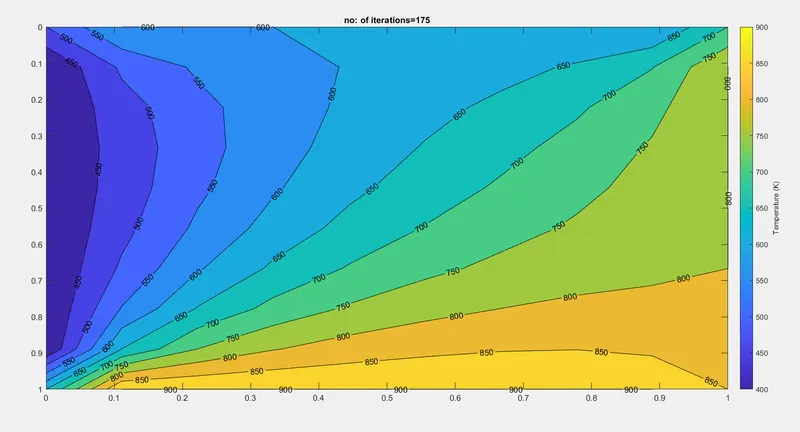
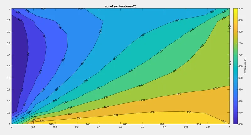
Steady state heat conduction implicit method:
Jacobi iteration
Gauss-seidel iteration:
SOR iteration:
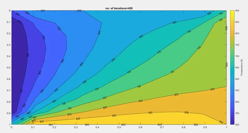
Transient State Analysis-Explicit:
Transient State Analysis-IMPLICIT:
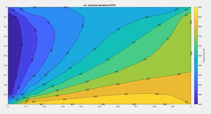
Jacobi Iteration:
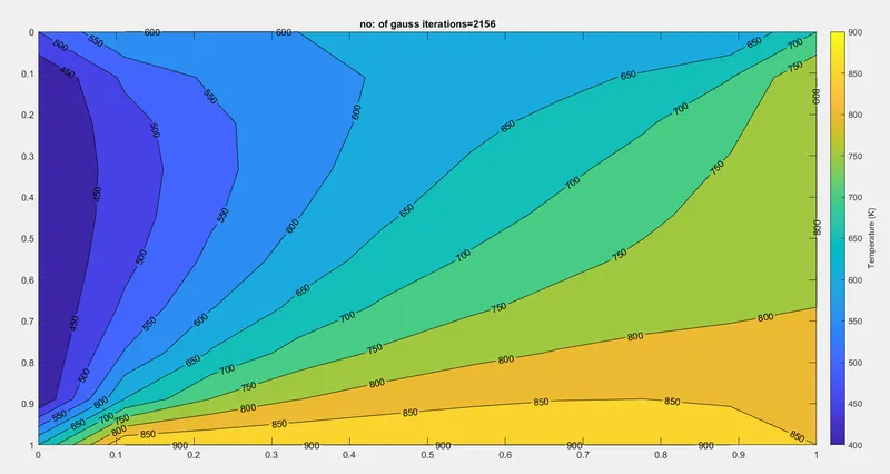
Gauss-seidel iteration:
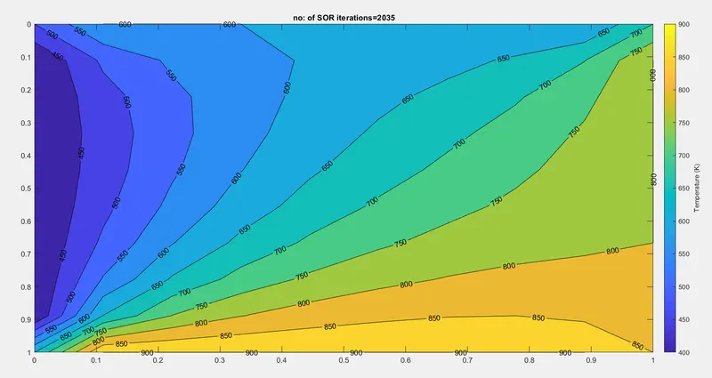
SOR Iteration:
Results :
Scheme Iteration Type Number of iterations
Steady State- Implicit Jacobi 207
Gauss-Siedel 175
SOR 76
Transient State-Implicit Jacobi 2703
Gauss-Siedel 2156
SOR 2035
Transient state-Explicit 428
CONCLUSION:
Finally, we obtained the results and contour plots, it can be concluded that the number of iterations follow the order Jacobi>Gauss-Seidel>SOR. Among the three iterative methods, SOR is better, as the number of iterations was less than Jacobi and Gauss-Seidel, for both steady and transient states.