Week 5.1 - Mid term project - Solving the steady and unsteady 2D heat conduction problem

SOLVING THE STEADY AND UNSTEADY 2D HEAT CONDUCTION PROBLEM

OBJECTIVE:

To perform Steady-state analysis & Transient State Analysis and solve the 2D heat conduction equation using the iterative point technique.

The Boundary conditions are as follows;

Top Boundary = 600 K

Bottom Boundary = 900 K

Left Boundary = 400 K

Right Boundary = 800 K

To implement the following methods for solving implicit equations.

1. Jacobi

2. Gauss-seidel

3. Successive over-relaxation

The absolute error criteria are 1e-4

To write code for both implicit and explicit schemes (for the Transient Analysis only).

THEORY:

Fluid flow and its properties can be solved and understood with the use of steady and unsteady analyses. We shall compute these analyses for the two-dimensional heat conduction problem in the current research. Heat transfer is the movement of thermal energy from one body that is hot to another that is cold. Both steady-state and non-steady-state circumstances can lead to this thermal energy transfer. There is only three-dimensional heat conduction in reality; there is no two-dimensional heat conduction. It is common practice to observe the flow and its parameters in 2-D using the 2-D heat conduction study. The heat equation is a partial differential equation that explains how the distribution of a certain quantity, like heat, changes over time in a solid medium as it naturally flows from higher temperature areas to lower temperature areas.

The heat equation for a function u(x, y, t) comprising two spatial variables (x, y) and the time variable t is,

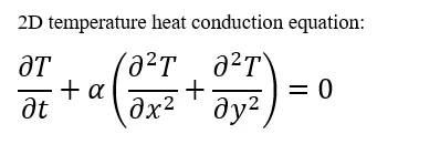
where `alpha` is the Thermal Diffusivity. Heat Conduction Techniques could take place under two circumstances,

1) steady-state - A Fluid state in which there is no change in the fluid property with respect to time is known as a Steady State.

2) transient or unsteady state - The unsteady or transient states contrast with steady states. Steady-state conditions are preceded by an unstable state. Under steady-state conditions, no system exists at first. After heat transmission begins, some time must pass before the system reaches a steady-state. The system is in an unsteady state during that transitional time.

MATLAB CODES:

A MATLAB code for getting inputs from the user and calling the required function code is given below:

%Week 5.1 - Solving the steady and unsteady 2D heat conduction problem
clear all 
close all 
clc

%X and Y
%number of x and y terms
nx = 10;
ny = 10;
%x and y
x = linspace(0,1,nx);
y = linspace(0,1,ny);


%TEMPERATURE
%initialising temperature values
T = 300 * ones(nx,ny);
%boundary conditions
T_L = 400;
T_T = 600;
T_R = 800;
T_B = 900;
%applying boundary conditions
T( 2:nx-1 , 1 ) = T_L;
T( 1 , 2:ny-1 ) = T_T;
T( 2:nx-1 , ny ) = T_R;
T( nx , 2:ny-1 ) = T_B;
%corner points
T(1,1) = (T_L + T_T) / 2;
T(1,ny) = (T_T + T_R) / 2;
T(nx,ny) = (T_R + T_B) / 2;
T(nx,1) = (T_B + T_L) / 2;


%making a copy of T
T_initial = T;

%inputs
omega = 1.4; %over relaxation factor
dt = 1e-2; % difference in time steps
alpha = 0.3; %thermal diffusivity
t = 5; %time in seconds


%selection of state
fprintf("2D TEMPERATURE HEAT CONDUCTION EQUATION \n")
fprintf("\nSelect a state \n");
fprintf("1)Steady State \t 2)Transient or Unsteady State \n");
state = input('\n(Expected input is 1 or 2)\n\nState = ');

%code for steady state
if state == 1
    fprintf("\nSTEADY STATE\n");
    fprintf("IMPLICIT SCHEME\n");
    fprintf("\nSelect a Method \n");
    fprintf("1)Jacobi Method \t 2)Gauss Seidel Method \t 3)Successive Over-Relaxation(SOR)-Gauss Seidel Method\n"); 
    method = input('\n(Expected input is 1,2 or 3)\n\nMethod = ');
    
    %code for implicit scheme
    if method == 1
        fprintf("\nSelected STEADY STATE -> IMPLICIT SCHEME -> JACOBI METHOD\n");
        [T_end] = ss_is_j(x,y,nx,ny,T);
    
    elseif method == 2
        fprintf("\nSelected STEADY STATE -> IMPLICIT SCHEME -> GAUSS SEIDEL METHOD\n");
        [T] = ss_is_gs(x,y,nx,ny,T);
        
    elseif method == 3
        fprintf("\nSelected STEADY STATE -> IMPLICIT SCHEME -> SOR-GAUSS SEIDEL METHOD\n");
        [T] = ss_is_sor(x,y,nx,ny,T,omega);
        
    else
        fprintf("\nINVALID INPUT\n");
    end
    
%code for transient state    
elseif state == 2
    fprintf("\nTRANSIENT STATE\n");
    fprintf("\nSelect a Method \n");
    fprintf("1)Implicit Scheme \t 2)Explicit Scheme\n");
    scheme = input('\n(Expected input is 1 or 2)\n\nScheme = ');
    
    %code for implicit scheme
    if scheme == 1
        fprintf("IMPLICIT SCHEME\n");
        fprintf("\nSelect a Method \n");
        fprintf("1)Jacobi Method \t 2)Gauss Seidel Method \t 3)Successive Over-Relaxation(SOR)-Gauss Seidel Method\n"); 
        method = input('\n(Expected input is 1,2 or 3)\n\nMethod = ');
        
        if method == 1
            fprintf("\nSelected TRANSIENT STATE -> IMPLICIT SCHEME -> JACOBI METHOD\n");
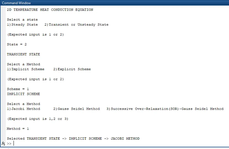
            [T] = ts_is_j(x,y,nx,ny,T,t,dt,alpha);
            
        elseif method == 2
            fprintf("\nSelected TRANSIENT STATE -> IMPLICIT SCHEME -> GAUSS SEIDEL METHOD\n");
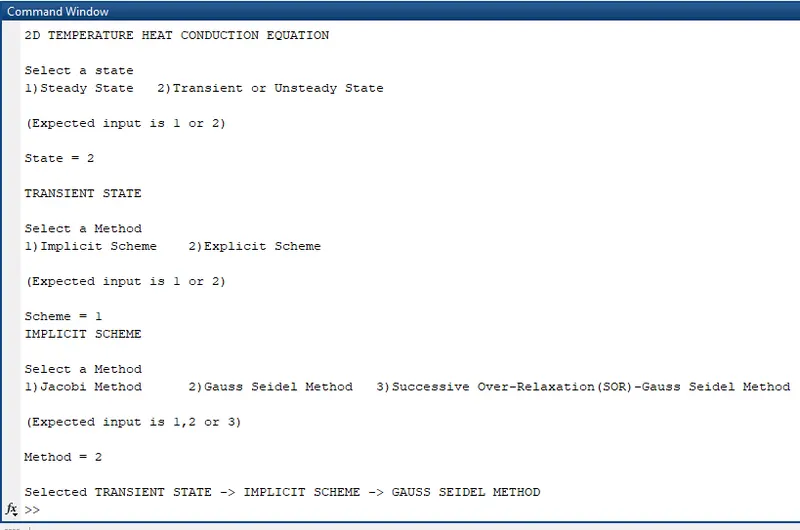
            [T] = ts_is_gs(x,y,nx,ny,T,t,dt,alpha);
            
        elseif method == 3
            fprintf("\nSelected TRANSIENT STATE -> IMPLICIT SCHEME -> SOR-GAUSS SEIDEL METHOD\n");
            [T] = ts_is_sor(x,y,nx,ny,T,t,dt,alpha,omega);
            
        else
            fprintf("\nINVALID INPUT\n");
        end
        
    %code for explicit scheme
    elseif scheme == 2
        fprintf("EXPLICIT SCHEME\n");
        fprintf("\nSelect a Method \n");
        fprintf("1)Jacobi Method \t 2)Gauss Seidel Method \t 3)Successive Over-Relaxation(SOR)-Gauss Seidel Method\n"); 
        method = input('\n(Expected input is 1,2 or 3)\n\nMethod = ');
        
        if method == 1
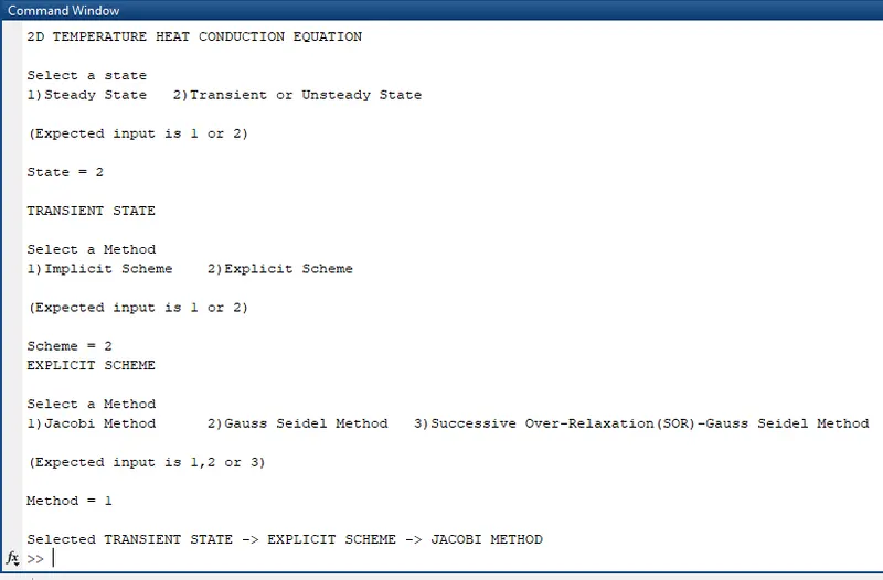
            fprintf("\nSelected TRANSIENT STATE -> EXPLICIT SCHEME -> JACOBI METHOD\n");
            [T] = ts_es_j(x,y,nx,ny,T,t,dt,alpha);
            
        elseif method == 2
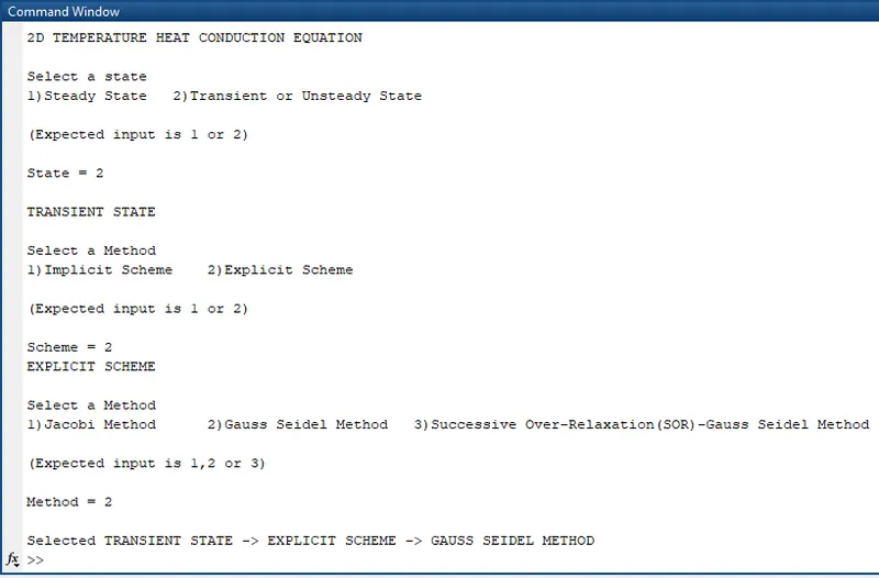
            fprintf("\nSelected TRANSIENT STATE -> EXPLICIT SCHEME -> GAUSS SEIDEL METHOD\n");
            [T] = ts_es_gs(x,y,nx,ny,T,t,dt,alpha);
            
        elseif method == 3
            fprintf("\nSelected TRANSIENT STATE -> EXPLICIT SCHEME -> SOR-GAUSS SEIDEL METHOD\n");
            [T] = ts_es_sor(x,y,nx,ny,T,t,dt,alpha,omega);
            
        else
            fprintf("\nINVALID INPUT\n");
        end
        
    else
        fprintf("\nINVALID INPUT\n");    
    end
    
else
    fprintf("\nINVALID INPUT\n");
end

• The sub-codes were created so that only the required parts are processed, which increases the efficiency of the code.
• Various states, schemes, and methods can be selected to view their specific solutions.
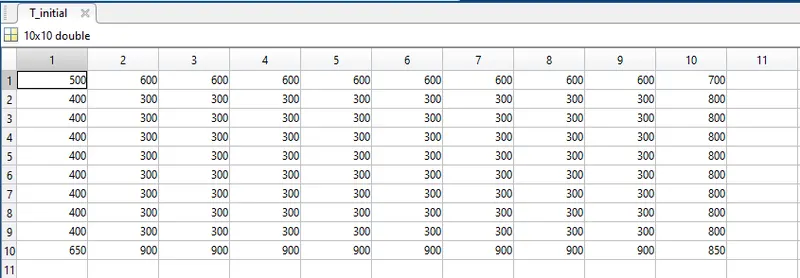
• The initial Temperature matrix with the given boundary conditions and refined boundary values is shown below,

STEADY-STATE:

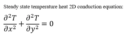
STEADY STATE -> Implicit scheme:

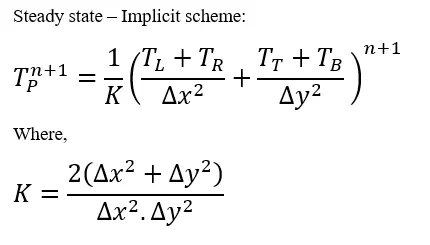
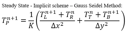
The equation for the steady-state Implicit scheme is given below,

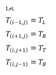
For better understanding,

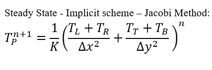
Jacobi method:

The appropriate MATLAB function code is given below,

function [T] = ss_is_j(x,y,nx,ny,T)
tic
%finding the dx and dy terms
dx = abs(x(2) - x(1));
dy = abs(y(2) - y(1));

%making a copy of T
T_old = T;

%others inputs
error = 9e9;
tol = 1e-4;
k = 2*((dx^2 + dy^2)/(dx^2*dy^2));
loop_no = 1;

while (error > tol)
    for i = 2 : nx-1
        for j = 2 : ny-1
            term_1 = (T_old(i-1,j) + T_old(i+1,j)) / (k*dx^2);
            term_2 = (T_old(i,j+1) + T_old(i,j-1)) / (k*dy^2);
            T(i,j) = term_1 + term_2;
        end
    end
    error = max( max( abs(T - T_old)));
    T_old = T;
    loop_no = loop_no + 1;
end
time_taken = toc;
contourf(x,y,T,'ShowText','on')
colormap(jet);
colorbar;
xlabel('X')
ylabel('Y')
title_1 = sprintf("Number of Iterations = %d", loop_no);
title_2 = sprintf("Simulation Time = %f s", time_taken);
title({"STEADY STATE -> IMPLICIT SCHEME -> JACOBI METHOD";title_1;title_2})
end

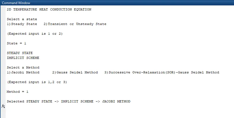
The inputs fed to the main code are state = 1 and method = 1

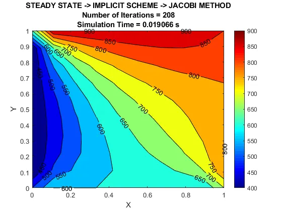
The obtained Contour plot is given below,

Gauss-Seidel method:

The appropriate MATLAB function code is given below,

function [T] = ss_is_gs(x,y,nx,ny,T)
tic
%finding the dx and dy terms
dx = abs(x(2) - x(1));
dy = abs(y(2) - y(1));

%making a copy of T
T_old = T;

%others inputs
error = 9e9;
tol = 1e-4;
k = 2*((dx^2 + dy^2)/(dx^2*dy^2));
loop_no = 1;

while (error > tol)
    for i = 2 : nx-1
        for j = 2 : ny-1
            term_1 = (T(i-1,j) + T_old(i+1,j)) / (k*dx^2);
            term_2 = (T_old(i,j+1) + T(i,j-1)) / (k*dy^2);
            T(i,j) = term_1 + term_2;
        end
    end
    error = max( max( abs(T - T_old)));
    T_old = T;
    loop_no = loop_no + 1;
end
time_taken = toc;
contourf(x,y,T,'ShowText','on')
colormap(jet);
colorbar;
xlabel('X')
ylabel('Y')
title_1 = sprintf("Number of Iterations = %d", loop_no);
title_2 = sprintf("Simulation Time = %f s", time_taken);
title({"STEADY STATE -> IMPLICIT SCHEME -> GAUSS SEIDEL METHOD";title_1;title_2})
end

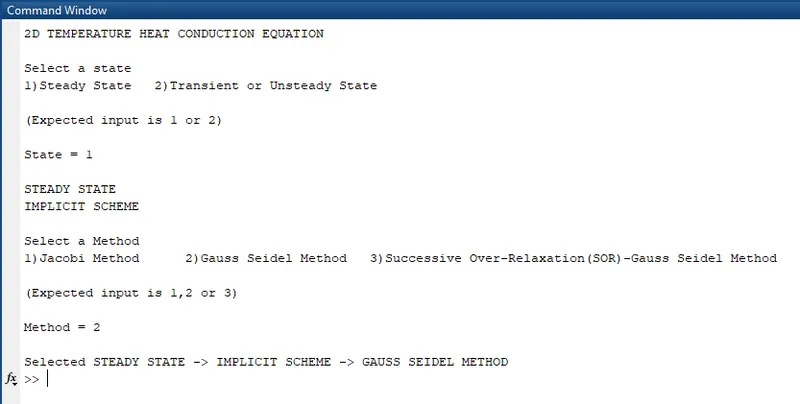
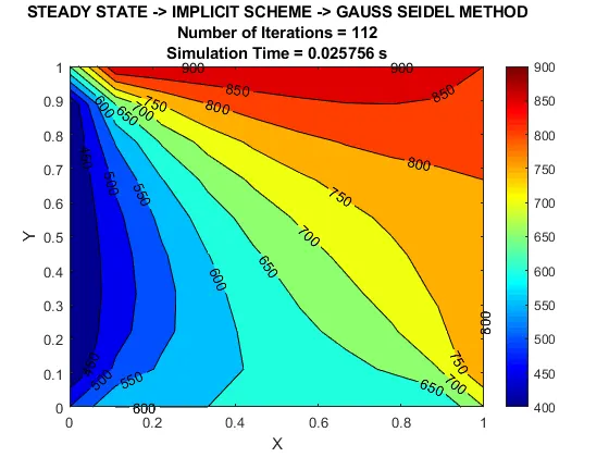
The inputs fed to the main code are state = 1 and method = 2

The obtained Contour plot is given below

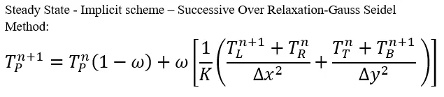
Successive Over Relaxation (SOR):

The appropriate MATLAB function code is given below,

function [T] = ss_is_sor(x,y,nx,ny,T,omega)
tic
%finding the dx and dy terms
dx = abs(x(2) - x(1));
dy = abs(y(2) - y(1));

%making a copy of T
T_old = T;

%others inputs
error = 9e9;
tol = 1e-4;
k = 2*((dx^2 + dy^2)/(dx^2*dy^2));
loop_no = 1;

while (error > tol)
    for i = 2 : nx-1
        for j = 2 : ny-1
            term_1 = (T(i-1,j) + T_old(i+1,j)) / (k*dx^2);
            term_2 = (T_old(i,j+1) + T(i,j-1)) / (k*dy^2);
            T(i,j) = (T_old(i,j)*(1-omega)) + omega*(term_1 + term_2);
        end
    end
    error = max( max( abs(T - T_old)));
    T_old = T;
    loop_no = loop_no + 1;
end
time_taken = toc;
contourf(x,y,T,'ShowText','on')
colormap(jet);
colorbar;
xlabel('X')
ylabel('Y')
title_1 = sprintf("Number of Iterations = %d", loop_no);
title_2 = sprintf("Simulation Time = %f s", time_taken);
title({"STEADY STATE -> IMPLICIT SCHEME -> SOR-GAUSS SEIDEL METHOD";title_1;title_2})
end

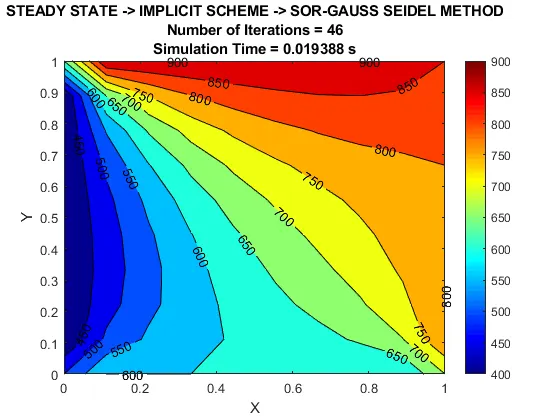
The inputs fed to the main code are state = 1 and method = 3

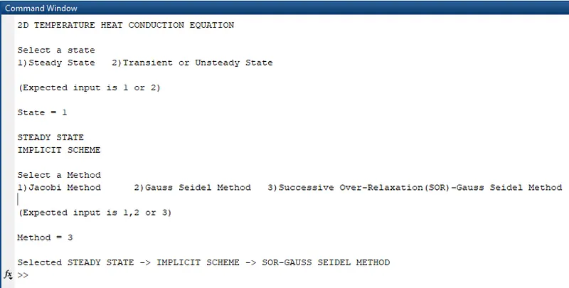
The obtained Contour plot is given below

TRANSIENT-STATE:

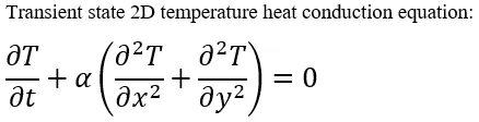
TRANSIENT STATE -> Implicit scheme:

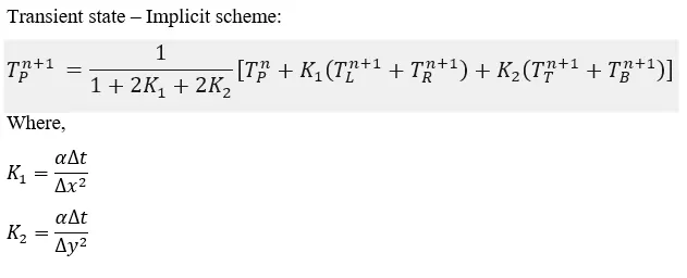
The equation for the unsteady-state Implicit scheme is given below,

Jacobi method:

The appropriate MATLAB function code is given below,

function [T] = ts_is_j(x,y,nx,ny,T,t,dt,alpha)
tic
%finding the dx and dy terms
dx = abs(x(2) - x(1));
dy = abs(y(2) - y(1));

%making a copy of T
T_old = T;
T_initial = T;

%others inputs
%error = 9e9;
tol = 1e-4;
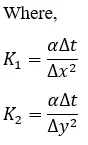
k_1 = (alpha*dt)/dx^2;
k_2 = (alpha*dt)/dy^2;
loop_no = 1;
nt = t/dt;

for m = 1 : nt
    error = 9e9;
    while (error > tol)
    for i = 2 : nx-1
        for j = 2 : ny-1
            k_term = 1 / (1+ (2*k_1) + (2*k_2) );
            term_1 = k_1 * (T_old(i-1,j) + T_old(i+1,j));
            term_2 = k_2 * (T_old(i,j+1) + T_old(i,j-1)) ;
            T(i,j) = k_term * (T_initial(i,j) + term_1 + term_2);
        end
    end
    error = max( max( abs(T - T_old)));
    T_old = T;
    loop_no = loop_no + 1;
    end
    T_initial = T;
end    
time_taken = toc;
contourf(x,y,T,'ShowText','on')
colormap(jet);
colorbar;
xlabel('X')
ylabel('Y')
title_1 = sprintf("Number of Iterations = %d", loop_no);
title_2 = sprintf("Simulation Time = %f s", time_taken);
title({"TRANSIENT STATE -> IMPLICIT SCHEME -> JACOBI METHOD";title_1;title_2})

end

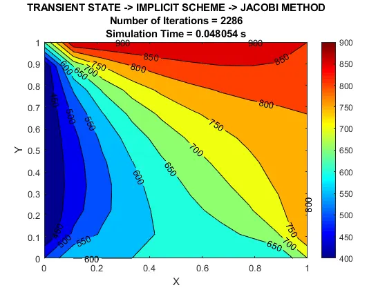
The inputs fed to the main code are state = 2, scheme = 1 and method = 1

The obtained Contour plot is given below

Gauss-Seidel method:

The appropriate MATLAB function code is given below,

function [T] = ts_is_gs(x,y,nx,ny,T,t,dt,alpha)
tic
%finding the dx and dy terms
dx = abs(x(2) - x(1));
dy = abs(y(2) - y(1));

%making a copy of T
T_old = T;
T_initial = T;

%others inputs
%error = 9e9;
tol = 1e-4;
k_1 = (alpha*dt)/dx^2;
k_2 = (alpha*dt)/dy^2;
loop_no = 1;
nt = t/dt;

for m = 1 : nt
    error = 9e9;
    while (error > tol)
    for i = 2 : nx-1
        for j = 2 : ny-1
            k_term = 1 / (1+ (2*k_1) + (2*k_2) );
            term_1 = k_1 * (T(i-1,j) + T_old(i+1,j));
            term_2 = k_2 * (T_old(i,j+1) + T(i,j-1)) ;
            T(i,j) = k_term * (T_initial(i,j) + term_1 + term_2);
        end
    end
    error = max( max( abs(T - T_old)));
    T_old = T;
    loop_no = loop_no + 1;
    end
    T_initial = T;
end    
time_taken = toc;
contourf(x,y,T,'ShowText','on')
colormap(jet);
colorbar;
xlabel('X')
ylabel('Y')
title_1 = sprintf("Number of Iterations = %d", loop_no);
title_2 = sprintf("Simulation Time = %f s", time_taken);
title({"TRANSIENT STATE -> IMPLICIT SCHEME -> GAUSS SEIDEL METHOD";title_1;title_2})

end

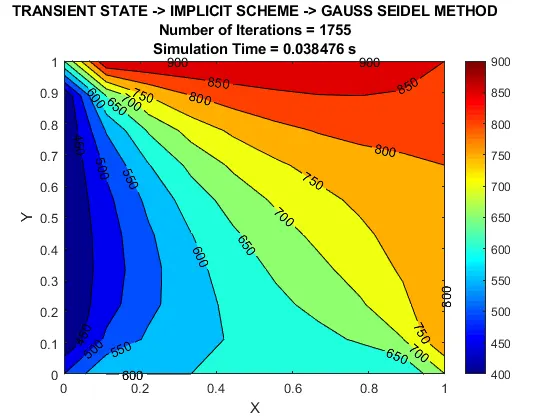
The inputs fed to the main code are state = 2, scheme = 1 and method = 2

The obtained Contour plot is given below

Successive Over Relaxation (SOR):

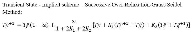
The appropriate MATLAB function code is given below,

function [T] = ts_is_sor(x,y,nx,ny,T,t,dt,alpha,omega)
tic
%finding the dx and dy terms
dx = abs(x(2) - x(1));
dy = abs(y(2) - y(1));

%making a copy of T
T_old = T;
T_initial = T;

%others inputs
%error = 9e9;
tol = 1e-4;
k_1 = (alpha*dt)/dx^2;
k_2 = (alpha*dt)/dy^2;
loop_no = 1;
nt = t/dt;

for m = 1 : nt
    error = 9e9;
    while (error > tol)
    for i = 2 : nx-1
        for j = 2 : ny-1
            k_term = 1 / (1+ (2*k_1) + (2*k_2) );
            term_1 = k_1 * (T(i-1,j) + T_old(i+1,j));
            term_2 = k_2 * (T_old(i,j+1) + T(i,j-1)) ;
            term_3 = omega*(k_term * (T_initial(i,j) + term_1 + term_2));
            T(i,j) = (T_initial(i,j)*(1-omega)) + term_3;
        end
    end
    error = max( max( abs(T - T_old)));
    T_old = T;
    loop_no = loop_no + 1;
    end
    T_initial = T;
end    
time_taken = toc;
contourf(x,y,T,'ShowText','on')
colormap(jet);
colorbar;
xlabel('X')
ylabel('Y')
title_1 = sprintf("Number of Iterations = %d", loop_no);
title_2 = sprintf("Simulation Time = %f s", time_taken);
title({"Selected TRANSIENT STATE -> IMPLICIT SCHEME -> SOR-GAUSS SEIDEL METHOD";title_1;title_2})

end

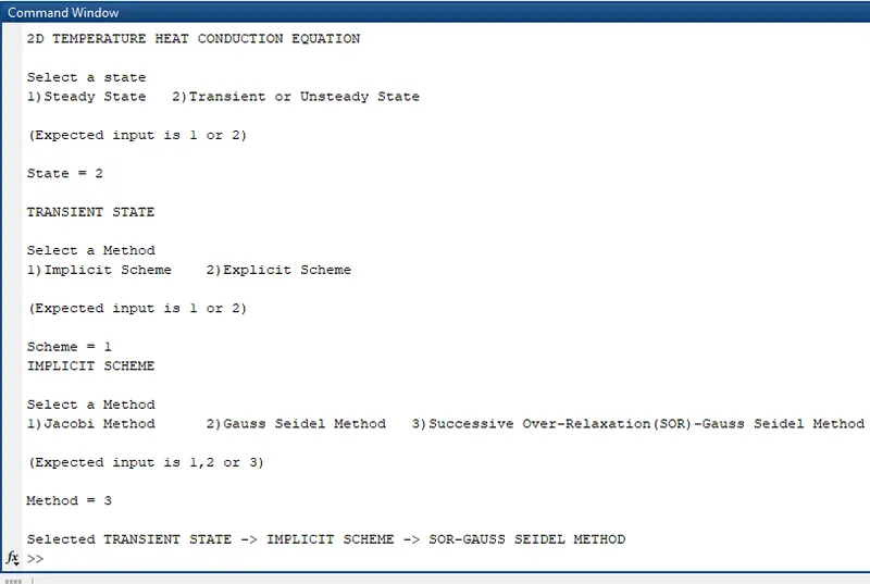
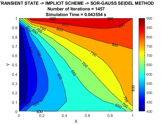
The inputs fed to the main code are state = 2, scheme = 1 and method = 3

The obtained Contour plot is given below

TRANSIENT STATE -> Explicit scheme:

The equation for the unsteady-state Explicit scheme is given below,

Jacobi method:

The appropriate MATLAB function code is given below,

function [T] = ts_es_j(x,y,nx,ny,T,t,dt,alpha)
tic
%finding the dx and dy terms
dx = abs(x(2) - x(1));
dy = abs(y(2) - y(1));

%making a copy of T
T_old = T;

%others inputs
%error = 9e9;
tol = 1e-4;
k_1 = (alpha*dt)/dx^2;
k_2 = (alpha*dt)/dy^2;
loop_no = 1;
nt = t/dt;

for m = 1 : nt
    error = 9e9;
    while (error > tol)
    for i = 2 : nx-1
        for j = 2 : ny-1
            term_1 = k_1 * (T_old(i-1,j) - 2*(T_old(i,j)) + T_old(i+1,j));
            term_2 = k_2 * (T_old(i,j+1) - 2*(T_old(i,j)) + T_old(i,j-1)) ;
            T(i,j) = T_old(i,j) + term_1 + term_2;
        end
    end
    error = max( max( abs(T - T_old)));
    T_old = T;
    loop_no = loop_no + 1;
    end
    
end    
time_taken = toc;
contourf(x,y,T,'ShowText','on')
colormap(jet);
colorbar;
xlabel('X')
ylabel('Y')
title_1 = sprintf("Number of Iterations = %d", loop_no);
title_2 = sprintf("Simulation Time = %f s", time_taken);
title({"TRANSIENT STATE -> EXPLICIT SCHEME -> JACOBI METHOD";title_1;title_2})

end

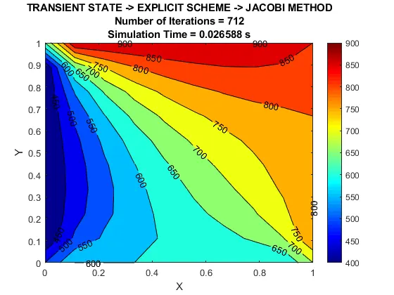
The inputs fed to the main code are state = 2, scheme = 2 and method = 1

The obtained Contour plot is given below

Gauss-Seidel method:

The appropriate MATLAB function code is given below,

function [T] = ts_es_gs(x,y,nx,ny,T,t,dt,alpha)
tic
%finding the dx and dy terms
dx = abs(x(2) - x(1));
dy = abs(y(2) - y(1));

%making a copy of T
T_old = T;

%others inputs
%error = 9e9;
tol = 1e-4;
k_1 = (alpha*dt)/dx^2;
k_2 = (alpha*dt)/dy^2;
loop_no = 1;
nt = t/dt;

for m = 1 : nt
    error = 9e9;
    while (error > tol)
    for i = 2 : nx-1
        for j = 2 : ny-1
            term_1 = k_1 * (T(i-1,j) - 2*(T_old(i,j)) + T_old(i+1,j));
            term_2 = k_2 * (T_old(i,j+1) - 2*(T_old(i,j)) + T(i,j-1)) ;
            T(i,j) = T_old(i,j) + term_1 + term_2;
        end
    end
    error = max( max( abs(T - T_old)));
    T_old = T;
    loop_no = loop_no + 1;
    end
    
end    
time_taken = toc;
contourf(x,y,T,'ShowText','on')
colormap(jet);
colorbar;
xlabel('X')
ylabel('Y')
title_1 = sprintf("Number of Iterations = %d", loop_no);
title_2 = sprintf("Simulation Time = %f s", time_taken);
title({"TRANSIENT STATE -> EXPLICIT SCHEME -> GAUSS SEIDEL METHOD";title_1;title_2})

end

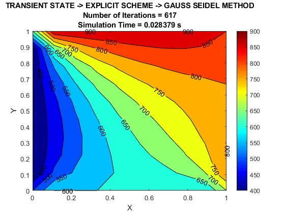
The inputs fed to the main code are state = 2, scheme = 2 and method = 2

The obtained Contour plot is given below

Successive Over Relaxation (SOR):

The appropriate MATLAB function code is given below,

function [T] = ts_es_sor(x,y,nx,ny,T,t,dt,alpha,omega)
tic
%finding the dx and dy terms
dx = abs(x(2) - x(1));
dy = abs(y(2) - y(1));

%making a copy of T
T_old = T;

%others inputs
%error = 9e9;
tol = 1e-4;
k_1 = (alpha*dt)/dx^2;
k_2 = (alpha*dt)/dy^2;
loop_no = 1;
nt = t/dt;

for m = 1 : nt
    error = 9e9;
    while (error > tol)
    for i = 2 : nx-1
        for j = 2 : ny-1
            term_1 = k_1 * (T(i-1,j) - 2*(T_old(i,j)) + T_old(i+1,j));
            term_2 = k_2 * (T_old(i,j+1) - 2*(T_old(i,j)) + T(i,j-1)) ;
            term_3 = omega * (T_old(i,j) + term_1 + term_2);
            T(i,j) = (T_old(i,j) * (1 - omega)) + term_3;
        end
    end
    error = max( max( abs(T - T_old)));
    T_old = T;
    loop_no = loop_no + 1;
    end
    
end    
time_taken = toc;
contourf(x,y,T,'ShowText','on')
colormap(jet);
colorbar;
xlabel('X')
ylabel('Y')
title_1 = sprintf("Number of Iterations = %d", loop_no);
title_2 = sprintf("Simulation Time = %f s", time_taken);
title({"TRANSIENT STATE -> EXPLICIT SCHEME -> SOR-GAUSS SEIDEL METHOD";title_1;title_2})

end

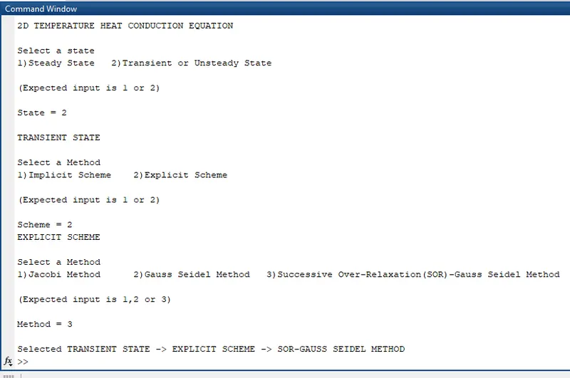
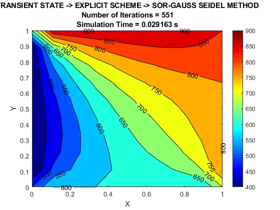
The inputs fed to the main code are state = 2, scheme = 2 and method = 3

The obtained Contour plot is given below

CONCLUSION:

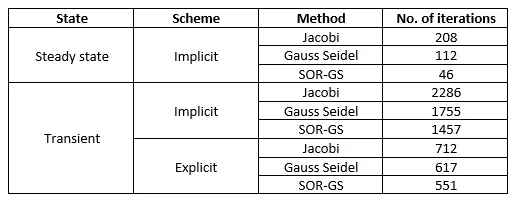
The 2D heat conduction equation for both steady-state and transient-state was solved using various methods and the results were plotted successfully. The Successive Over-Relaxation method has the best results for the analysis as it has the lowest possible iterations. The over-relaxation factor can be varied to find an accurate solution easily in the SOR method.