Week 11 - Simulation of Flow through a pipe in OpenFoam
Simulation of Flow through a pipe in OpenFoam
Aim: To simulate the axi symmetric flow in a pipe through openfoam.
Objective:
- Validate Hydro-dynamic length with the numerical result
- Validate the fully developed flow velocity profile with its analytical profile
- Validate maximum velocity and pressured drop for fully developed flow
- Post-process Shear stress and validate wall shear stress for fully developed flow
Solution:
Consider the water flow through the pipe of 20 mm diameter at velocity of 0.0935m/s of Reynold's number less than 2100, hence laminar flow. Due to No-slip condition, fluid particles in contact with the pipe stops completely.
Boundary layer theory:
Consider a fluid entering a circular pipe at uniform velocity, with no-slip condition.
The velocity of fluid at mid-section has to increase to keep mass flow rate through the pipe constant, resulting in velocity gradient.
Hydrodynamic entrance region is region from inlet to the point at which velocity profile becomes fully developed, and its length is hydrodynamic entrance length.
Reynolds number is the ratio of inertial force to viscous force.
`Re=rho*v*L/mu`
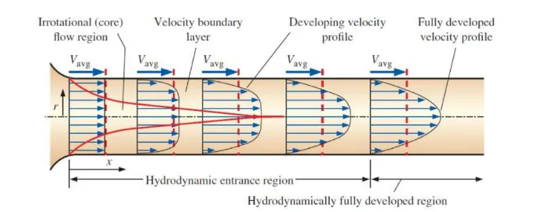
Hagen- Poiseuille's flow: It is the pressure drop in incompressible fluid in laminar flow through the long cylindrical pipe of constant cross section. Flow is caused to flow by pressure difference between the points, from higher pressure to lower pressure.
It is assumed to have no acceleration of flow. Flow resistance offered is shear stress.
Shear stress is `tau=mu*(du)/(dy)`
pressure difference is represented as
`deltap=(32*mu*V*L)/D^2`
Enterance length
L_ent=0.06*Re*D
Matlab code:
clear all
close all
clc

D=0.02;
Re=2100;
rho=1000; %density
theta=4;
nu=8.91e-7;  %kinematic viscocity

%dynamic vis
mu=rho*nu;
v_avg= mu*Re/(rho*D);
v_max=2*v_avg;

L_w=0.3;
L_entrance= 0.06* Re*D;
L=L_entrance+L_w;


%pressure drop in flow
delta_p= 32*mu*v_avg*L_w/D^2;


r=D/2;
R=linspace(0,r,500);1.

for i=1:length(R)

    tau(i)=2*mu*v_max*(abs(R(i)))/r^2;

end

for j=1: length(R)

    vel_p(j)=2*v_avg*(1-(abs(R(j))^2/r^2));
end
figure(1)
plot(R,tau)
ylabel('shear stress')
xlabel('Radial length')

figure (2)
plot(R,vel_p)
ylabel('velocity')
xlabel('Radial length')
%blockmeshdict file

v0=[0 0 0];
v1=[0 r*cosd(theta/2) -r*sind(theta/2)];
v2=[0 r*cosd(theta/2) r*sind(theta/2)];
v3=[L 0 0];
v4=[L r*cosd(theta/2) -r*sind(theta/2)];
v5=[L r*cosd(theta/2) r*sind(theta/2)];

f1=fopen('blockMeshDict','w');

fprintf(f1,'\t FoamFile \n')
fprintf(f1,'\t { \n')
fprintf(f1,'\t \t format      ascii;\n')
fprintf(f1,'\t\t class       dictionary;\n')
fprintf(f1,'\t\t object      blockMeshDict;\n')
fprintf(f1,'\t } \n')
%vertices
fprintf(f1,'%s \n','convertToMeters 1 ;')
fprintf(f1,'\n %s \n','vertices')
fprintf(f1,'%s \n','(')
fprintf(f1,'\t(%d %d %d)\n',v0(1), v0(2), v0(3))
fprintf(f1,'\t(%d %d %d)\n',v1(1), v1(2), v1(3))
fprintf(f1,'\t(%d %d %d)\n',v2(1), v2(2), v2(3))
fprintf(f1,'\t(%d %d %d)\n',v3(1), v3(2), v3(3))
fprintf(f1,'\t(%d %d %d)\n',v4(1), v4(2), v4(3))
fprintf(f1,'\t(%d %d %d)\n',v5(1), v5(2), v5(3))
fprintf(f1,'%s \n',');')

%blocks
fprintf(f1,'%s \n','blocks')
fprintf(f1,'%s \n','(')
fprintf(f1,'\t hex(0 3 4 1 0 3 5 2) (%d %d %d) simpleGrading (%d %d %d)\n', 200,20,1,1,0.1,1)
fprintf(f1,'%s \n',');')

%edges
fprintf(f1,'\n %s \n','edges')
fprintf(f1,'%s \n','(')
fprintf(f1,'\t arc 1 2 (%d %d %d) \n',0,r,0)
fprintf(f1,'\t arc 1 2 (%d %d %d) \n',L,r,0)
fprintf(f1,'\n %s',');')

%boundary
fprintf(f1,'\n %s \n','boundary')
fprintf(f1,'%s \n','(')
fprintf(f1,'\n %s \n','axis')
fprintf(f1,'{ \n \t type empty; \n')
fprintf(f1,'\t faces \n( \n')
fprintf(f1,'\t (%d %d %d %d) \n',0,3,3,0)
fprintf(f1,'\t ) ; \n }\n')

%wall
fprintf(f1,'\n %s \n','wall')
fprintf(f1,'%s \n','{')
fprintf(f1,'\t type wall; \n')
fprintf(f1,'\t faces \n ( \n')
fprintf(f1,'\t (%d %d %d %d) \n',1,4,5,2)
fprintf(f1,'\t ) ; \n }\n')

%inlet
fprintf(f1,'\n %s \n','inlet')
fprintf(f1,'%s \n','{')

fprintf(f1,'\t type patch; \n')
fprintf(f1,'\t faces \n ( \n')
fprintf(f1,'\t (%d %d %d %d) \n',0,1,2,0)
fprintf(f1,'\t ) ; \n }\n')

%outlet
fprintf(f1,'\n %s \n','outlet')
fprintf(f1,'%s \n','{')
fprintf(f1,'\t type patch; \n')
fprintf(f1,'\t faces \n ( \n')
fprintf(f1,'\t (%d %d %d %d) \n',3,5,4,3)
fprintf(f1,'\t ); \n }\n')

%front
fprintf(f1,'\n\t front \n { \n')
fprintf(f1,'\t type wedge ; \n')
fprintf(f1,'\t faces \n ( \n')
fprintf(f1,'\t (%d %d %d %d) \n',0,3,4,1)
fprintf(f1,'\t ) ; \n \t }\n')

%back
fprintf(f1,'\n\t back \n { \n')
fprintf(f1,'\t type wedge ; \n')
fprintf(f1,'\t faces \n ( \n')
fprintf(f1,'\t (%d %d %d %d) \n',0,2,5,3)
fprintf(f1,'\t ) ; \n \t }\n')

fprintf(f1,');')
Explaination:
1. Assign the initial values of the Hagen-Pousville flow.
2. Calculating the properties like dynamic viscocity, average velocity, maximum velocity, entrance length.
3. Change in pressure `delta p`
4. Calculate the shear stress and velocity profile by for loop.
5. Plotting the values to obtain analytical solution.
Create BlockMeshDict file by using write function:
1. Assign vertices at all points on the wedge. (v1, v2 ,v3 , v4, v5)
2. Drafting the blockMeshDict file using write function in MATLAB.
3. Drafting should be made with similar pattern as per the blockMeshDict file used in openFoam.
4. Writing the vertices of the wedge.
5. Creating the hexagonal block with grading factor of 0.1 along Y-axis (finer mesh near walls).
6. Assigning edges, wall, boundary, inlet, outlet, front and back of blocks.
Procedure to simulate the flow:
a. To select solver and copy folder
1. Open terminal command in ubuntu.
2. open tutorials, code: tut
3. And open incompressible folder and select icofoam, then cavity. (code: icoFoam)
4. Copy cavity folder to run folder. using code: 'cp -r pipr/$FOAM_RUN'
5. Type run command to open run folder.
6. Open pipe. (code: cd pipe)
(6a. Also copy and paste the blockMeshDict file created by MATLAB in system folder)
7. Open system file.
8. Run blockMeshDict code file. (code: blockMesh)
BlockMeshDict file:
FoamFile
{
    format      ascii;
    class       dictionary;
    object      blockMeshDict;
}
convertToMeters 1 ;

 vertices
(
	(0 0 0)
	(0 9.993908e-03 -3.489950e-04)
	(0 9.993908e-03 3.489950e-04)
	(2.820000e+00 0 0)
	(2.820000e+00 9.993908e-03 -3.489950e-04)
	(2.820000e+00 9.993908e-03 3.489950e-04)
);
blocks
(
	 hex (0 3 4 1 0 3 5 2) (200 20 1) simpleGrading (1 0.1 1)
);

 edges
(
	 arc 1 2 (0 1.000000e-02 0)
	 arc 4 5 (2.820000e+00 1.000000e-02 0)

 );
 boundary
(

 axis
{
 	 type empty;
	 faces
(
	 (0 3 3 0)
	 ) ;
 }

 wall
{
	 type wall;
	 faces
 (
	 (1 4 5 2)
	 ) ;
 }

 inlet
{
	 type patch;
	 faces
 (
	 (0 1 2 0)
	 ) ;
 }

 outlet
{
	 type patch;
	 faces
 (
	 (3 5 4 3)
	 );
 }

	 front
 {
	 type wedge ;
	 faces
 (
	 (0 3 4 1)
	 ) ;
 	 }

	 back
 {
	 type wedge ;
	 faces
 (
	 (0 2 5 3)
	 ) ;
 	 }
);
ControlDict file:
/*--------------------------------*- C++ -*----------------------------------*\
  =========                 |
  \\      /  F ield         | OpenFOAM: The Open Source CFD Toolbox
   \\    /   O peration     | Website:  https://openfoam.org
    \\  /    A nd           | Version:  9
     \\/     M anipulation  |
\*---------------------------------------------------------------------------*/
FoamFile
{
    format      ascii;
    class       dictionary;
    location    "system";
    object      controlDict;
}
// * * * * * * * * * * * * * * * * * * * * * * * * * * * * * * * * * * * * * //

application     icoFoam;

startFrom       startTime;

startTime       5;

stopAt          endTime;

endTime         15;

deltaT          0.05;

writeControl    runTime;

writeInterval   0.1;

purgeWrite      10;

writeFormat     ascii;

writePrecision  6;

writeCompression off;

timeFormat      general;

timePrecision   6;

runTimeModifiable true;


// ************************************************************************* //
Eplaination:
1. open control dict file in system folder (code: gedit controlDict).
2. Assign start time as 5 and end time 15, delta t 0.05.
p and U files:
p file:
1. Open 0 folder in block_test
(code: cd..
code :cd 0)
2. Open files p file( code: gedit p)
code for p:
/*--------------------------------*- C++ -*----------------------------------*\
  =========                 |
  \\      /  F ield         | OpenFOAM: The Open Source CFD Toolbox
   \\    /   O peration     | Website:  https://openfoam.org
    \\  /    A nd           | Version:  9
     \\/     M anipulation  |
\*---------------------------------------------------------------------------*/
FoamFile
{
    format      ascii;
    class       volScalarField;
    object      p;
}
// * * * * * * * * * * * * * * * * * * * * * * * * * * * * * * * * * * * * * //

dimensions      [0 2 -2 0 0 0 0];

internalField   uniform 0;

boundaryField
{
    outlet
    {
        type            fixedValue;
        value           uniform 0;
    }
    inlet
    {
        type            zeroGradient;
    }
    axis
    {
        type            empty;
    }

    wall
    {
        type            zeroGradient;
    }

    front
    {
        type            wedge;
    }
    back
    {
        type            wedge;
    }
}

// ************************************************************************* //
1. Assign outlet as uinform 0.
2. Inlet and oulet as zerogradient, front and back as wedge.
Open file U file( code: gedit U)
/*--------------------------------*- C++ -*----------------------------------*\
  =========                 |
  \\      /  F ield         | OpenFOAM: The Open Source CFD Toolbox
   \\    /   O peration     | Website:  https://openfoam.org
    \\  /    A nd           | Version:  9
     \\/     M anipulation  |
\*---------------------------------------------------------------------------*/
FoamFile
{
    format      ascii;
    class       volVectorField;
    object      U;
}
// * * * * * * * * * * * * * * * * * * * * * * * * * * * * * * * * * * * * * //

dimensions      [0 1 -1 0 0 0 0];

internalField   uniform (0.0936 0 0);

boundaryField
{
    inlet
    {
        type            fixedValue;
        value           uniform (0.0936 0 0);
    }
    outlet
    {
        type            zeroGradient;
    }
    axis
    {
        type            empty;
    }

    wall
    {
        type            noSlip;
    }

    front
    {
        type            wedge;
    }
    back
    {
        type            wedge;
    }
}

// ************************************************************************* //
Explaination:
1. Assign outlet and fixedwalls as zero gradient.
2. Front and back as empty.
3. Inlet as uniform (0.0936 0 0) fixed value, obtained from MATLAB value.
Transient properties as :
1. Open constant foler
2. Open transientProperties file. (code: gedit transientProperties)
3. Give value nu = 8.91e-7 (Kinematic viscosity of water)
/*--------------------------------*- C++ -*----------------------------------*\
  =========                 |
  \\      /  F ield         | OpenFOAM: The Open Source CFD Toolbox
   \\    /   O peration     | Website:  https://openfoam.org
    \\  /    A nd           | Version:  9
     \\/     M anipulation  |
\*---------------------------------------------------------------------------*/
FoamFile
{
    format      ascii;
    class       dictionary;
    location    "constant";
    object      transportProperties;
}
// * * * * * * * * * * * * * * * * * * * * * * * * * * * * * * * * * * * * * //

nu              [0 2 -1 0 0 0 0] 8.91e-7;


// ************************************************************************* //
Open paraview:
1. Change directory to block_test
2. Run code: checkMesh
3. Run code:icoFoam
4. Run code: paraFoam
5. In paraview click apply.
Results and discussion:
Paraview:
Geometry of wedge:
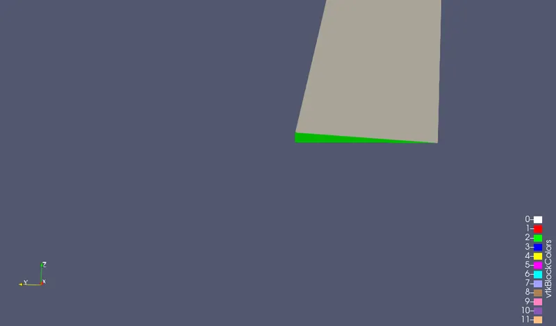
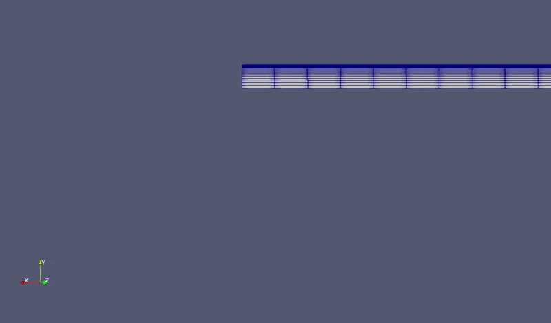
Blockmesh:
Select options 'surface with edges' and 'solid color'
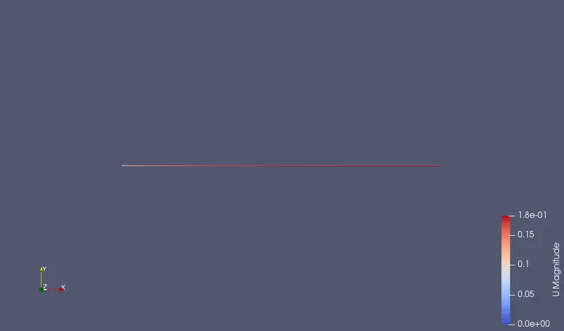
Geometry velocity profile:
Select option 'U'
Plots generated at different points:
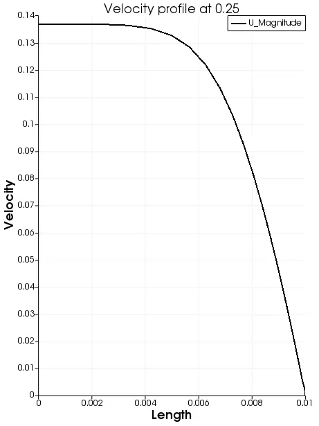
Velocity profile at 0.25
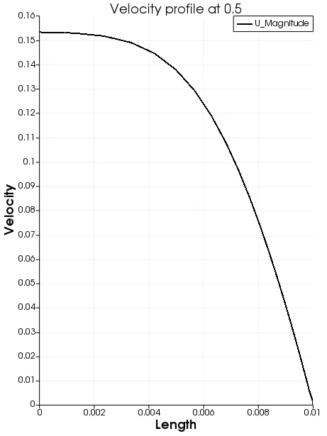
Velocity profile at 0.5
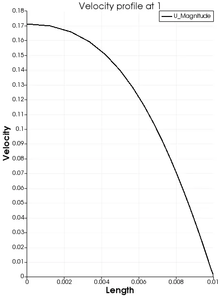
Velocity profile at 1
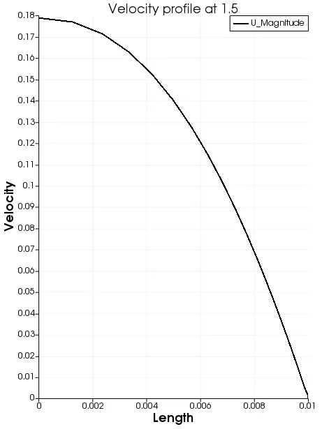
Velocity profile at 1.5
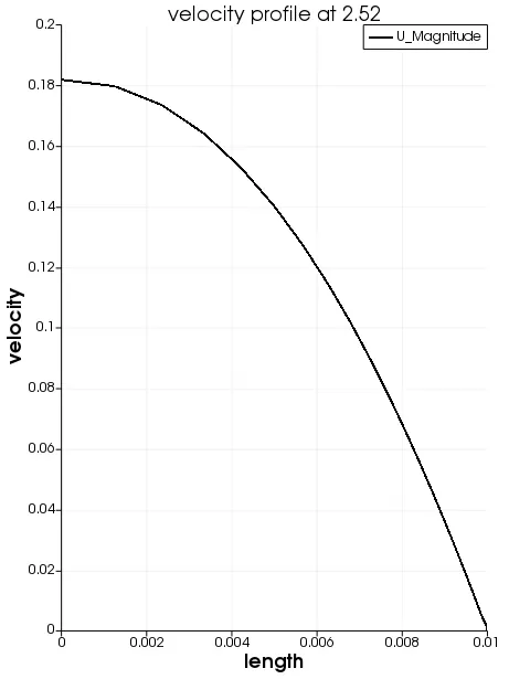
Velocity profile at entrance length (2.52)
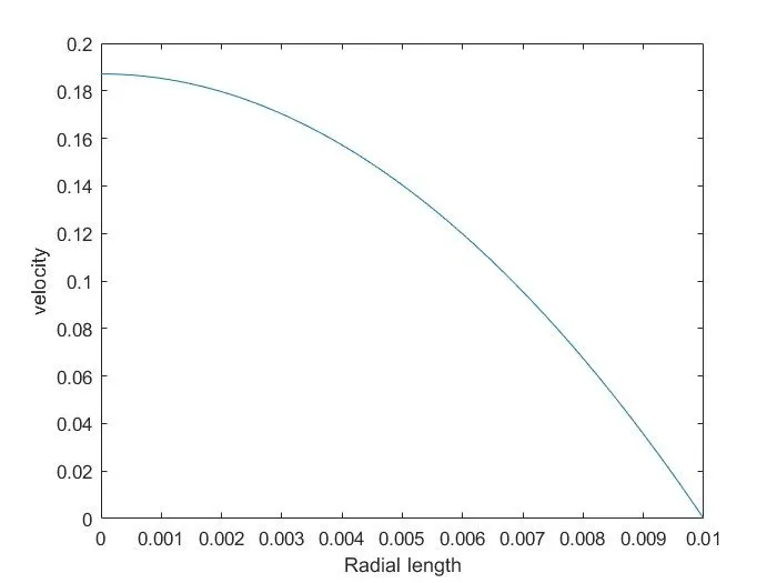
The Analytical velocity profile obtained from the Matlab :
Shear stress:
Shear stress is deformation of material by slippage along a plane.
Mathematical expression: `tau=mu*(du)/(dy)`
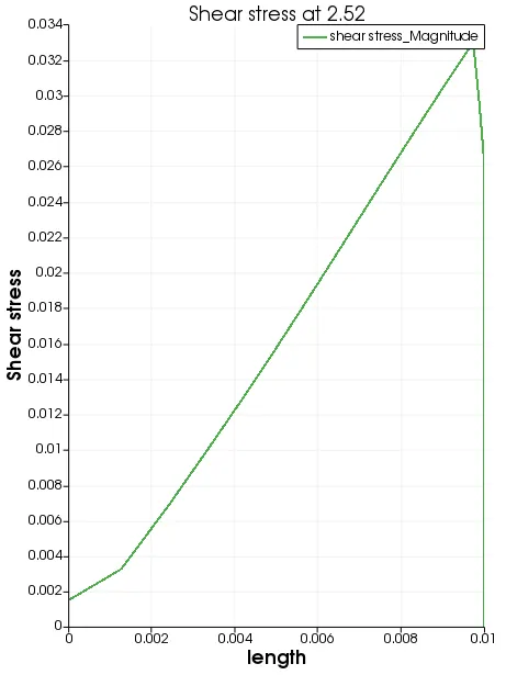
Shear stress graph of fully developed flow:
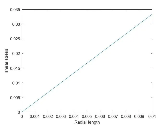
Analytical shear stress graph obtained by MATLAB:
Pressure drop:
Pressure drop graph of fully developed region.
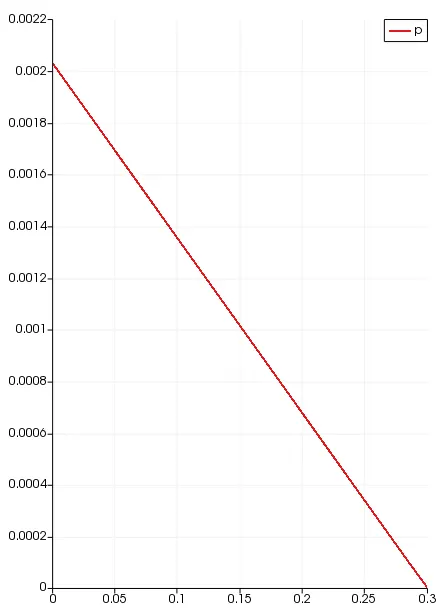
The value of point at 2.52 is 0.002031
The value of point at 2.82 is 4.53e-6
Difference between them is `gradp`= 0.002030547, obtained from the graph,
analytical value of pressure drop `grad p` =2.006 in mm.
Conclusion:
Hydro dynamic length is obtained to be 2.52 units, where velocity profile is fully developed.
The velocity profile gradually increase from inlet to outlet. It remains constant after the flow is fully developed.
Analytical velocity profile and velocity obtained in openfoam matches very well, where velocity is maximum at centre and parabolically decrease toward wall.
Shear stress is zero at centre of pipe and increases linearly toward the wall, graph obtained from openfoam is close to analytical result.
Maximum velocity and pressure drop value is obtained for fully develpoed flow.