Week 5.1 - Mid term project - Solving the steady and unsteady 2D heat conduction problem
- AIM:
The main aim of the project is to solve the steady and transient 2d heat conduction equation using iterative techniques.
- OBJECTIVE:
STEADY STATE ANALYSIS:
`(del^2T)/(delx^2)+(del^2T)/(dely^2)=0`,since this equation is in elliptical form can be discretize by using central differencing scheme
`(T_(i+1,j)-2T_(i,j)+T_(i-1,j))^n/(Deltax^2)+(T_(i,j+1)-2T_(i,j)+T_(i,j-1))^n/(Deltay^2)=0`
let `k=2*((Deltax^2+Deltay^2)/(Deltax^2*Deltay^2))`
then
`T_(i,j)=(1/k)*((T_(i-1,j)+T_(i+1,j))/(Deltax^2)+(T_(i,j-1)+T_(i,j+1))/(Deltay^2))`
For Jacobi iterative method,
`T_(i,j)^(n+1)=(1/k)*((T_(i-1,j)+T_(i+1,j))/(Deltax^2)+(T_(i,j-1)+T_(i,j+1))/(Deltay^2))^n`
For Gauss-seidel iterative method,
`T_(i,j)^(n+1)=(1/k)*((T_(i-1,j)+T_(i+1,j))/(Deltax^2)+(T_(i,j-1)+T_(i,j+1))/(Deltay^2))^(n+1)`
and for Succesive over relaxation iterative method,
`T_(i,j)^(n+1)=T_(i,j)^n*(1-omega)+omega*(1/k)*((T_(i-1,j)+T_(i+1,j))/(Deltax^2)+(T_(i,j-1)+T_(i,j+1))/(Deltay^2))^(n+1)`
- CODING:
%Solving steady  2D Heat conduction problem

clear all
close all
clc

%Initial conditions
L = 1;
nx = 10;
ny = 10;
x = linspace(0,1,nx);
y = linspace(0,1,ny);
dx = x(2)-x(1);
dy = y(2)-y(1);

%Providing Boundary and initial condition

t = 300*ones(nx,ny);
t(:,1)=400;
t(:,ny)=800;
t(1,:)=600;
t(nx,:)=900;

%Defining temperature at corner points
t(1,1)=500;
t(1,ny)=700;
t(nx,ny)=850;
t(nx,1)=650;

%Time step
dt=1e-2;
told = t;
error =100;
tol = 1e-4;
k = 2*(dx^2+dy^2)/(dx^2*dy^2);

%Input

method = input('Iterative method= ');

%Jacobi method

if method ==1
    tic;
    jacobi_iter=1;
    %Convergence loop
    while(error>tol)
        %Space loop
        for i=2:(nx-1)
            for j=2:(ny-1)
                term1 = (1/k)*((told(i-1,j)+told(i+1,j))/(dx^2));
                term2 = (1/k)*((told(i,j-1)+told(i,j+1))/(dy^2));
                t(i,j)=term1+term2;
            end
        end
        error = max(max(abs(t-told)));
        told = t;%Updating the t value
        jacobi_iter = jacobi_iter+1;
        time_taken = toc;
    end

    %Plotting
    figure(1)
    contourf(x,y,t,'ShowText','on')
    colormap(jet);
    colorbar;
    xlabel('X')
    ylabel('Y')
    set(gca,'Ydir','reverse')
    text1 = sprintf('Number of iteration = %d',jacobi_iter);
    text2 = sprintf('Simulation time=%f',time_taken);
    title({'Steady state heat conduction profile by jacobi iteration';text1;text2});
end

%Gauss-Seidal iterative method

if(method==2)
    tic;
    gauss_iter=1;
    %Convergence loop
    while(error>tol)
        %Space loop
        for i=2:(nx-1)
            for j=2:(ny-1)
                term1 = (1/k)*((t(i-1,j)+told(i+1,j))/(dx^2));
                term2 = (1/k)*((t(i,j-1)+told(i,j+1))/(dy^2));
                t(i,j)=term1+term2;
            end
        end
        error = max(max(abs(t-told)));
        told = t;%Updating the t value
        gauss_iter = gauss_iter+1;
        time_taken = toc;
    end

    %Plotting
    figure(1)
    contourf(x,y,t,'ShowText','on')
    colormap(jet);
    colorbar;
    xlabel('X')
    ylabel('Y')
    set(gca,'Ydir','reverse')
    text1 = sprintf('Number of iteration = %d',gauss_iter);
    text2 = sprintf('Simulation time=%f',time_taken);
    title({'Steady state heat conduction profile by Gauss-Seidal iterative method';text1;text2});
end

%Successive over relaxation method

if(method==3)
    tic;
    sor_iter=1;
    omega=1.3;
    while(error>tol)
        for i = 2:(nx-1)
            for j =2:(ny-1)
                term1 = (1/k)*(t(i-1,j)+told(i+1,j))/(dx^2);
                term2 = (1/k)*(t(i,j-1)+told(i,j+1))/(dy^2);
                t(i,j)=((1-omega)*told(i,j))+(omega*(term1+term2));
            end
        end
        error = max(max(abs(t-told)));
        told = t;
        sor_iter = sor_iter+1;
        time_taken=toc;
    end
     %Plotting
    figure(1)
    contourf(x,y,t,'ShowText','on')
    colormap(jet);
    colorbar;
    xlabel('X')
    ylabel('Y')
    set(gca,'Ydir','reverse')
    text1 = sprintf('Number of iteration = %d',sor_iter);
    text2 = sprintf('Simulation time=%f',time_taken);
    title({'Steady state heat conduction profile by Successive over relaxation method';text1;text2});
end- EXPLANATION:
- Start the code by providing initial condition like domain length L,number of nodes in x and y axis and use linspsace comand to generate x and y length with nx and ny number of nodes.
- Assume the temperature inside the domain as 300k and provide the boundary temperature values.
- Input the corner point temperature values as an average of the adjacent node temperature values.
- Define the time step and initial error and provide the tolerance value.
- Input iterative method required by the user should enter to solve the steady state analysis.
- tic and toc command is used to find the simulation time.
- If user enter the value as '1' ,jacobi iterative method will be in use to solve the Steady state analysis.
- Inside the convergence loop,space loop should be specified and after evaluating error the old temperature value should be updated.
- Plotting should be done using contourf comand.
- OUTPUT:
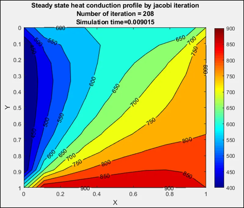
FOR JACOBI ITERATIVE METHOD:
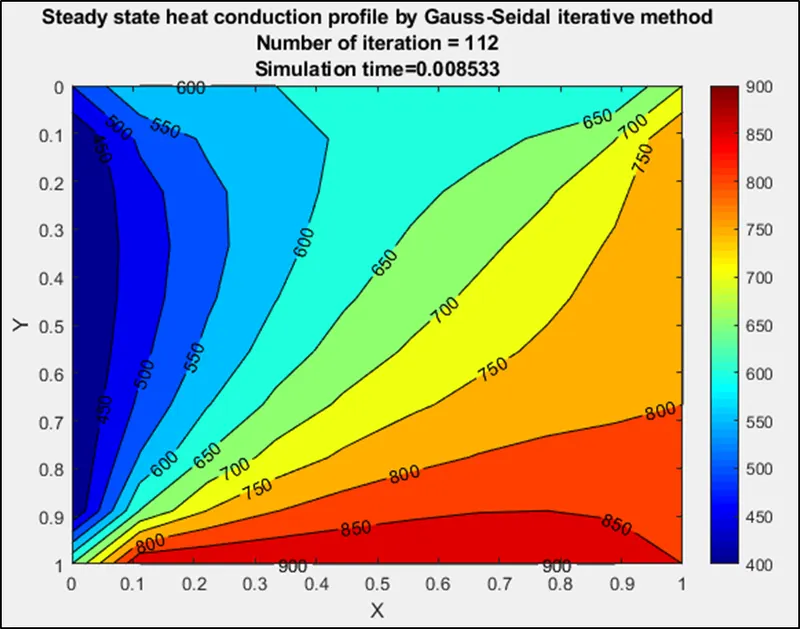
FOR GAUSS-SEIDEL ITERATIVE METHOD:
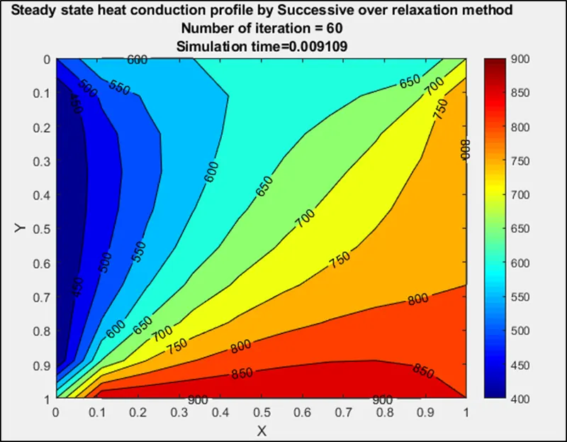
FOR SUCESSIVE OVER RELAXATION METHOD:
- CONCLUSION:
From the above plots it is clear that number of iteration for jacobi method>Gauss-seidel method>SOR method.
TRANSIENT(UNSTEADY ) STATE ANALYSIS:
IMPLICIT APPROCH:
`(del^2T)/(delx^2)+(del^2T)/(dely^2)=1/(alpha)*(delT)/(delt)` is unsteady form of 2D heat conduction equation
LHS side can be discretize using Central differencing scheme and `(delT)/(delt)` can be discretize using first-order forward differencing scheme
we get,
`((T_(i+1,j)-2T_(i,j)+T_(i-1,j))/(Deltax^2)+(T_(i,j+1)-2T_(i,j)+T_(i,j-1))/(Deltay^2))=1/(alpha)*(T_(i,j)^(n+1)-T_(i,j)^n)/(Deltat)`
let `k_1=alpha*((Deltat)/(Deltax^2))` and `k_2=alpha*((Deltat)/(Deltay^2))`
Now by rearranging we get,
`T_(i,j)^(n+1)=(T_(i,j)^n+K_1(T_(i+1,j)+T_(i-1,j))^(n+1)+K_2(T_(i,j+1)+T_(i,j-1))^(n+1))/(1+2k_1+2k_2)`
For jacobi iterative method,
`T_(i,j)^(n+1)=(T_(i,j)^n+K_1(T_(i+1,j)+T_(i-1,j))^(n)+K_2(T_(i,j+1)+T_(i,j-1))^(n))/(1+2k_1+2k_2)`
For Gauss-siedal iterative method
`T_(i,j)^(n+1)=(T_(i,j)^n+K_1(T_(i+1,j)+T_(i-1,j))^(n+1)+K_2(T_(i,j+1)+T_(i,j-1))^(n+1))/(1+2k_1+2k_2)`
For sucessive over Relaxation iterative method,
`T_(i,j)^(n+1)=(1-omega)*T_(i,j)^n+omega*((T_(i,j)^n+K_1(T_(i+1,j)+T_(i-1,j))^(n+1)+K_2(T_(i,j+1)+T_(i,j-1))^(n+1))/(1+2k_1+2k_2))`
- CODING:
%Solving Unsteady heat conduction problem with Implicit approch

clear all
close all
clc

%Initial conditions
L = 1;
nx = 10;
ny = 10;
nt = 1400;
x = linspace(0,1,nx);
y = linspace(0,1,ny);
dx = x(2)-x(1);
dy = y(2)-y(1);

%Providing Boundary and initial condition

t = 300*ones(nx,ny);
t(:,1)=400;
t(:,ny)=800;
t(1,:)=600;
t(nx,:)=900;

%Defining temperature at corner points
t(1,1)=500;
t(1,ny)=700;
t(nx,ny)=850;
t(nx,1)=650;

%Time step
dt=0.01;
told = t;
tol = 1e-4;

alpha = 0.3; %Thermal diffusivity
t_prev = told;

k1 = alpha*(dt/dx^2);
k2 = alpha*(dt/dy^2);

%Input

method = input('Iterative method= ');

%Jacobi method

if method ==1
    tic;
    jacobi_iter=1;
    %Time loop
    for k = 1:nt
        error = 100;
        %Convergence loop
        while(error>tol)
            %Space loop
            for i = 2:(nx-1)
                for j = 2:(ny-1)
                    term1 = 1/(1+2*k1+2*k2);
                    term2 = k1*term1;
                    term3 = k2*term1;
                    H = (told(i-1,j)+told(i+1,j));
                    V = (told(i,j-1)+told(i,j+1));
                    t(i,j)=((t_prev(i,j)*term1)+(term2*H)+(term3*V));
                end
            end
            error = max(max(abs(t-told)));
            told = t;
            jacobi_iter = jacobi_iter +1;
        end
        t_prev = t;
    end
    time_taken = toc;

     %Plotting
    figure(1)
    contourf(x,y,t,'ShowText','on')
    colormap(jet);
    colorbar;
    xlabel('X')
    ylabel('Y')
    set(gca,'Ydir','reverse')
    text1 = sprintf('Number of iteration = %d',jacobi_iter);
    text2 = sprintf('Simulation time=%f',time_taken);
    title({'Transient state heat conduction profile by jacobi iteration';text1;text2});
end

 %Gauss-Seidal iterative method

 if method ==2
    tic;
    gauss_iter=1;
    %Time loop
    for k = 1:nt
        error = 100;
        %Convergence loop
        while(error>tol)
            %Space loop
            for i = 2:(nx-1)
                for j = 2:(ny-1)
                    term1 = 1/(1+2*k1+2*k2);
                    term2 = k1*term1;
                    term3 = k2*term1;
                    H = (t(i-1,j)+told(i+1,j));
                    V = (t(i,j-1)+told(i,j+1));
                    t(i,j)=((t_prev(i,j)*term1)+(term2*H)+(term3*V));
                end
            end
            error = max(max(abs(t-told)));
            told = t;
            gauss_iter = gauss_iter +1;
        end
        t_prev = t;
    end
    time_taken = toc;

     %Plotting
    figure(1)
    contourf(x,y,t,'ShowText','on')
    colormap(jet);
    colorbar;
    xlabel('X')
    ylabel('Y')
    set(gca,'Ydir','reverse')
    text1 = sprintf('Number of iteration = %d',gauss_iter);
    text2 = sprintf('Simulation time=%f',time_taken);
    title({'Transient state heat conduction profile by Gauss iteration method';text1;text2});
end

%Successive over relaxation method

if(method==3)
    tic;
    sor_iter=1;
    omega=1.3;
     %Time loop
    for k = 1:nt
        error = 100;
        %Convergence loop
        while(error>tol)
            %Space loop
            for i = 2:(nx-1)
                for j = 2:(ny-1)
                    term1 = 1/(1+2*k1+2*k2);
                    term2 = k1*term1;
                    term3 = k2*term1;
                    H = (t(i-1,j)+told(i+1,j));
                    V = (t(i,j-1)+told(i,j+1));
                    t(i,j)= told(i,j)*(1-omega)+omega*(((t_prev(i,j)*term1)+(term2*H)+(term3*V)));
                end
            end
            error = max(max(abs(t-told)));
            told = t;
            sor_iter = sor_iter +1;
        end
        t_prev = t;
    end
    time_taken = toc;

     %Plotting
    figure(1)
    contourf(x,y,t,'ShowText','on')
    colormap(jet);
    colorbar;
    xlabel('X')
    ylabel('Y')
    set(gca,'Ydir','reverse')
    text1 = sprintf('Number of iteration = %d',sor_iter);
    text2 = sprintf('Simulation time=%f',time_taken);
    title({'Transient state heat conduction profile by Successive over relaxation method';text1;text2});
end
- EXPLANATION:
- Start the code by providing initial condition like domain length L,number of nodes in x and y axis and use linspsace comand to generate x and y length with nx and ny number of nodes.
- Assume the temperature inside the domain as 300k and provide the boundary temperature values.
- Input the corner point temperature values as an average of the adjacent node temperature values.
- Define the time step and initial error and provide the tolerance value and thermal diffusivity alpha value.
- Input iterative method required by the user should enter to solve the steady state analysis.
- tic and toc command is used to find the simulation time.
- If user enter the value as '1' ,jacobi iterative method will be in use to solve the Steady state analysis.
- For each time loop, convergence loop should run and then space loop should be specified and after evaluating error the old temperature value should be updated.
- Plotting should be done using contourf comand.
- OUTPUT:
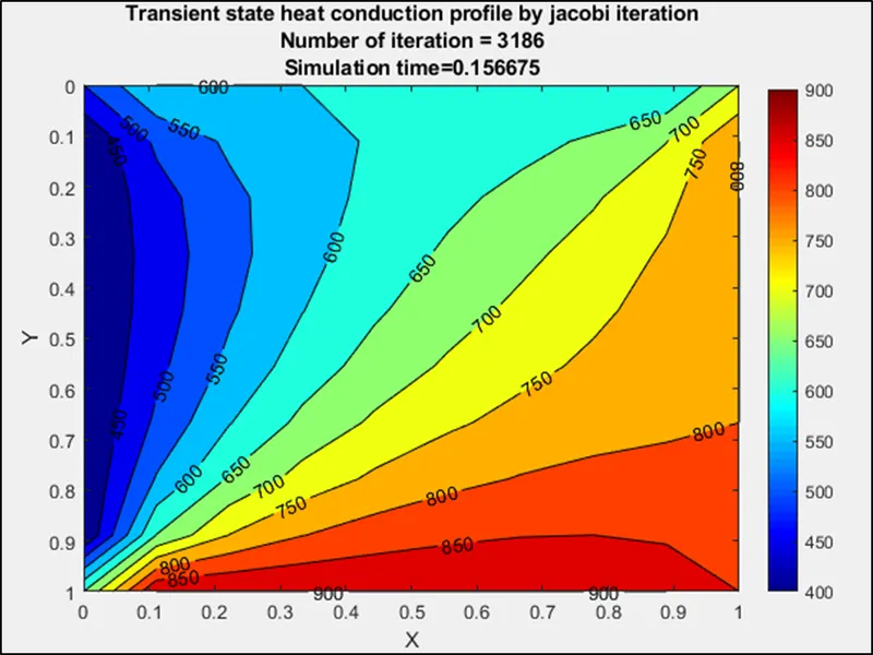
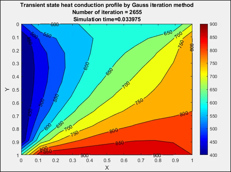
FOR JACOBI ITERATIVE METHOD:
FOR GAUSS-SEIDAL ITERATIVE METHOD:
FOR SUCESSIVE OVER RELAXATION ITERATIVE METHOD:
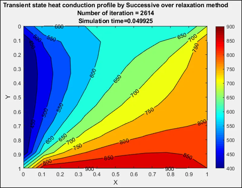
- CONCLUSION:
For unsteady state analysis number of iteration taken for jacobi method>Gauss-Siedal method>Sucessive over relaxation method,since we are using updated value of temperature in gauss siedal method we are getting less number of iteration compare to the jacobi iterative method,and we are using over relaxation factor of 1.3 so solution converge at faster iterative steps in SOR method than other two.
EXPLICIT APPROCH:
`(del^2T)/(delx^2)+(del^2T)/(dely^2)=1/(alpha)*(delT)/(delt)` is unsteady form of 2D heat conduction equation
`(T_(i,j)^(n+1)-T_(i,j)^n)/(Deltat)-alpha*((T_(i+1,j)-2T_(i,j)+T_(i-1,j))^n/(Deltax^2)+(T_(i,j+1)-2T_(i,j)+T_(i,j-1))^n/(Deltay^2)))=0`
`T_(i,j)^(n+1)=T_(i,j)^n+(alpha*Deltat)*(((T_(i+1,j)-2T_(i,j)+T_(i-1,j))^n/(Deltax^2)+(T_(i,j+1)-2T_(i,j)+T_(i,j-1))^n/(Deltay^2)))`
Let `k_1=alpha*(Deltat)/(Deltax^2)`
`k_2=alpha*(Deltat)/(Deltay^2)`
`T_(i,j)^(n+1)=T_(i,j)^n+k_1*(T_(i+1,j)-2T_(i,j)+T_(i-1,j))^n+(T_(i,j+1)-2T_(i,j)+T_(i,j-1))^n`
- CODING:
clear all
close all
clc

%Initial conditions
L = 1;
nx = 10;
ny = 10;
nt = 1400;
x = linspace(0,1,nx);
y = linspace(0,1,ny);
dx = x(2)-x(1);
dy = y(2)-y(1);

%Providing Boundary and initial condition

t = 300*ones(nx,ny);
t(:,1)=400;
t(:,ny)=800;
t(1,:)=600;
t(nx,:)=900;

%Defining temperature at corner points
t(1,1)=500;
t(1,ny)=700;
t(nx,ny)=850;
t(nx,1)=650;

%Time step
dt=0.01;
told = t;
tol = 1e-4;

alpha = 0.3; %Thermal diffusivity


%CFL numbers

k1 = alpha*(dt/dx^2);
k2 = alpha*(dt/dy^2);

%Time loop
tic
explicit_iter = 1;
for k = 1:nt
    %Space loop
    for i = 2:(nx-1)
       for j = 2:(ny-1)
            term1 = told(i+1,j)-2*told(i,j)+told(i-1,j);
            term2 = told(i,j+1)-2*told(i,j)+told(i,j-1);
            t(i,j)=told(i,j)+k1*term1+k2*term2;
        end
    end
    told=t;
    explicit_iter = explicit_iter+1;
end
time_taken=toc;
%Plotting
    figure(1)
    contourf(x,y,t,'ShowText','on')
    colormap(jet);
    colorbar;
    xlabel('X')
    ylabel('Y')
    set(gca,'Ydir','reverse')
    text1 = sprintf('Number of iteration = %d',explicit_iter);
    text2 = sprintf('Simulation time=%f',time_taken);
    title({'Transient state heat conduction profile by explicit approch';text1;text2});
- OUTPUT:
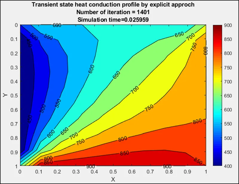
- CONCLUSION:
Steady state and Transient state analysis for 2D heat conduction problem using iterative method has be coded using MATLAB and plots has been plotted for various methods and simulation time for each method has been noted.