Week 5.1 - Mid term project - Solving the steady and unsteady 2D heat conduction problem

Midterm project - Solving the steady and unsteady 2D heat conduction problem

AIM: Solve the 2D heat conduction equation by using the point iterative techniques that were taught in the class.

OBJECTIVE:

• Solve the 2D heat conduction equation by using the point iterative techniques that were taught in the class.

• You will implement the following methods for solving implicit equations.

  1. Jacobi

  2. Gauss-seidel

  3. Successive over-relaxation

• Your absolute error criteria are 1e-4

• You will write code for both implicit and explicit schemes (This is for the Transient Analysis only)

THEORY:

The given condition for the 2D HEAT CONDUCTION EQUATION

`(delT)/(delt)=alpha((del^2T)/(del^2x)+(del^2T)/(del^2y))`

METHODS

Explicit method: This method, calculates the system status at a future time from the currently known system status.

In the explicit methods, iterative methods are not used, because all values are known values. Just substituting known values in the equation will get solutions.

Implicit method: This method calculates the system status at a future time from the system statuses at present and future times.

In the implicit method, iterative methods are used, because all unknown values are presented.

Iterative methods:

An iterative method is a mathematical procedure that uses an initial guess to generate a sequence of improving approximate solutions for a class of problems, in which the n-th approximation is derived from the previous ones.

Jacobi method:

Jacobi method is an iterative method where all updated values are used for the computations only after all the variables have been updated.

Gauss-Seidel method:

Gauss-Seidel method is an iterative method, where the updated variables are used in the computations as
soon as they are updated.

Successive over-Relaxation (SOR):

SOR is a variant of the Gauss-Seidel method for solving a system of linear equations, resulting in faster convergence. It is also used for slowly converging iterative processes.

If relaxation factor <1 then the method is under-relaxed.

relaxation factor >1 then the method is over-relaxed.

As for STEADY STATE:

we know that

`frac{∂ T}{∂ t} = 0`

so the equation becomes,

`(∂^2T)/(∂x^2)+(∂^2T)/(∂y^2) = 0`

Discretizing the above equation

`(del^2T)/(delx^2) = (T_(i-1,j)-2T_(i,j)+T_(i+1,j))/(Deltax^2)`

`(del^2T)/(dely^2) = (T_(i,j-1)-2T_(i,j)+T_(i,j+1))/(Deltay^2)`

So the equation becomes,

`(T_(i-1,j)-2T_(i,j)+T_(i+1,j))/(Deltax^2) + (T_(i,j-1)-2T_(i,j)+T_(i,j+1))/(Deltay^2) = 0`

As Nx=Ny, we consider `Deltax = Deltay`

on rearranging the terms we get

`T_(i,j) = 1/4(T_(i-1,j)+T_(i+1,j)+T_(i,j-1)+T_(i,j+1))`

GIVEN:

Top Boundary = 600 K

Bottom Boundary = 900 K

Left Boundary = 400 K

Right Boundary = 800 K

CODE AND EXPLANATION:

MAIN CODE

1. We start by specifying the number of grid points in the spatial domain x and y-direction. In this case, is 10 grid points in the x and y-direction.

2. Then we specify the length of the x and y space domain.

3. And Defining the spatial domain for the length and grid points specified.

4. Then we calculating the grid spacing in the x and y space domain.

5. Defining temperature with the guess values for the number of the grid points defined.

6. By applying the Boundary Conditions as mentioned.

7. The accuracy of the solution is measured with the computed approximated solution and compared with the tolerance value so that the converged solution is in the desired accuracy.

8. Calculating `K`, `K_1, and K_2`. Here `alpha` is taken 1.4`

9. We call the function to calculate the temperature values at n+1 time step for both steady and unsteady state using different iterative solvers and an explicit method is also used for calculating temperature for unsteady-state heat conduction equation.

Explanation of Functions

• In the functions, dummy error is assigned to the error variable so that the while loop condition would satisfy and iterations are calculated.
• The error is calculated and updated for each iteration. The error calculated is coded to take only the absolute values since negative values will not satisfy the while loop condition and iterations will stop and the results obtained will not be a converged result.
• The number of iterations taken for the solution to converge is stored in the iter variable. This is done by incrementing the iter variable by 1 for each iteration.
• As the iteration proceeds to calculate the temperature at n+1 time step temperature at nth time step is required and these temperature values should be updated for each iteration. If the temperature values are not updated for each iteration the solution will not converge and while loop will run infinite times.
• Contourf plot is used to check if the solutions are converged or not i.e., the plot does not change as the approximated temperature value changes in the order of tolerance value defined.
• This logic is used in the below functions to calculate the temperature of the Steady-state Heat Conduction equation for the desired accuracy.

Solving the steady-state 2D Heat Conduction

clear all
close all
clc

% inputs
L = 1;
n_x = 20;
n_y = 20;
x = linspace(0,L,n_x);
y = linspace(0,L,n_y);
dx = x(2) - x(1);
dy = y(2) - y(1);
error = 9e9;
tol = 1e-4;

% boundary conditions
T_left = 400;
T_top = 600;
T_right = 800;
T_bottom = 900;
T = ones(n_x,n_y);
% Temperature at boundary
T(2:n_y - 1,1) = T_left;
T(2:n_y - 1,n_x) = T_right;
T(1,2:n_x - 1) = T_top;
T(n_x,2:n_y - 1) = T_bottom;
 
T(1,1) = (T_top + T_left)/2;
T(n_x,n_y) = (T_right + T_bottom)/2;
T(1,n_y) = (T_top + T_right)/2;
T(n_x,1) = (T_left + T_bottom)/2;

k1 = (dx^2)/(2*(dx^2 + dy^2));
k2 =( dy^2)/(2*(dx^2 + dy^2));

jacobi_iteration(T,x,y,n_x,n_y,tol,error,k1,k2)

gauss_iteration(T,x,y,n_x,n_y,tol,error,k1,k2);

sor_iteration(T,x,y,n_x,n_y,tol,error,k1,k2);

JACOBI-ITERATION

  %Jacobi Iteration
  function jacobi_iteration(T,x,y,n_x,n_y,tol,error,k1,k2)
    
    [X,Y] = meshgrid(x,y);
    T_old = T;
    tic
    jacobi_iteration = 1;
    while(error>tol)
    for i = 2:n_x - 1
      for j = 2:n_y - 1
        T(i,j) = k1*(T_old(i - 1,j) + T_old(i + 1,j))+k2*(T_old(i,j - 1) + T_old(i,j + 1));
      end
    end
    
    error = max(max(abs(T_old - T)));
    T_old = T;
    jacobi_iteration = jacobi_iteration + 1;
   end
  
  time = toc;
  figure(1)
  contourf(x,y,T);
  [a b] = contourf(x,y,T);
  clabel(a,b);
  xlabel('x-axis');
  ylabel('y-axis');
  colorbar
  hold on
  
  title_name = sprintf('No of Jacobi iteration = %d',jacobi_iteration);
  title(title_name)
  file = sprintf('Jacobi.png');
  saveas(gca,file);
  fprintf('Number of iteration %d \n',jacobi_iteration);
  fprintf('Time taken for solving equation is %f \n',time);
end

GAUSS-ITERATION

% Gauss iteration
function gauss_iteration(T,x,y,n_x,n_y,tol,error,k1,k2)
  
  [X,Y] = meshgrid(x,y);
  T_old = T;
  gauss_iteration = 2;
  while(error>tol)
  for i = 2:n_x - 1
    for j = 2:n_y-1
      T(i,j)=k1*(T(i,j - 1) + T_old(i,j + 1)) + k2*(T(i - 1,j) + T_old(i + 1,j));
    end
  end
  
  error = max(max(abs(T_old - T)));
  T_old = T;
  gauss_iteration = gauss_iteration + 1;
  end

time = toc;
figure(2)
contourf(x,y,T);
[a b] = contourf(x,y,T);
clabel(a,b);
xlabel('x-axis')
ylabel('y-axis')
hold on
colorbar

title_name = sprintf('No of Gauss iteration = %d',gauss_iteration);
title(title_name)
file = sprintf('gs.png');
saveas(gca,file);
fprintf('Number of iteration %d \n',gauss_iteration);
fprintf('Time taken for solving equation is %f \n',time);
end

SOR-ITERATION

function sor_iteration(T,x,y,n_x,n_y,tol,error,k1,k2)
  
  % relaxation factor calculation
  z = cos(pi/n_x) + cos(pi/n_y);
  omega = 4/(2 + sqrt(4 - z^2));
  T_old = T;
  [X,Y] = meshgrid(x,y);
  
  sor_iteration = 1;
  while(error>tol)
  for i = 2:n_x - 1
    for j = 2:n_y - 1
      T(i,j) = omega*(k1*(T(i,j - 1) + T(i,j + 1)) + k2*(T(i - 1,j) + T(i + 1,j))) + (1 - omega)*T_old(i,j);
    end
  end
  
  error = max(max(abs(T_old - T)));
  T_old = T;
  sor_iteration = sor_iteration + 1;
  end

time = toc;
figure(3)
contourf(x,y,T);
[a b] = contourf(x,y,T);
clabel(a,b);
xlabel('x-axis')
ylabel('y-axis')
hold on
colorbar

title_name = sprintf('no of SOR iteration = %d',sor_iteration);
title(title_name)
file = sprintf('S_SOR.png');
saveas(gca,file);
fprintf('Relaxation factor considered is %d \n',omega);
fprintf('Number of iterations %f \n',sor_iteration);
fprintf('Time taken for solving equation is %f \n',time);
end

RESULTS:

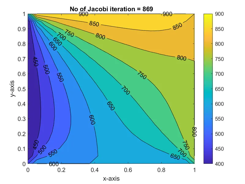
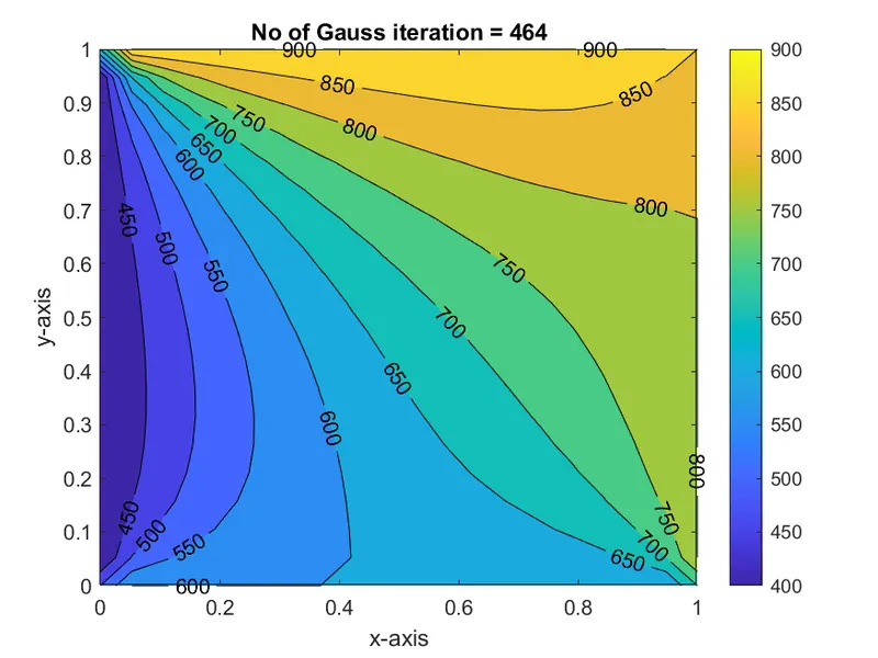
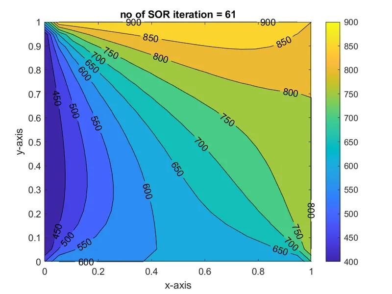
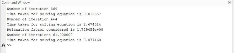
SNAP OF COMMAND WINDOW

So we conclude,

As we notice in the above graphs and results, the Gauss method has a high convergence rate while comparing to the Jacobi method and the Gauss method and SOR method has the same convergence rate because we assume relaxation factor w=1.

SNAP OF WORKSPACE

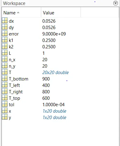
Solving Transient state 2D Heat Conduction Explicit Method

clear all
close all
clc

% Inputs
L=1;
n_x=20;
n_y=20;
x=linspace(0,L,n_x);
y=linspace(0,L,n_y);
dx=x(2)-x(1);
dy=y(2)-y(1);
dt=30;
nt=1000;
error=9e9;
tol=1e-4;

% boundary conditions
T_left = 400;
T_top = 600;
T_right = 800;
T_bottom=900;
T = ones(n_x,n_y);
% Temperature at boundary
T(2:n_y - 1,1) = T_left;
T(2:n_y - 1,n_x) = T_right;
T(1,2:n_x - 1) = T_top;
T(n_x,2:n_y - 1) = T_bottom;
 
T(1,1) = (T_top + T_left)/2;
T(n_x,n_y) = (T_right + T_bottom)/2;
T(1,n_y) = (T_top + T_right)/2;
T(n_x,1) = (T_left + T_bottom)/2;

alpha = 2.3e-5;
CFL = alpha*dt/(dx^2);

k4 = (alpha*dt)/(dx^2);
k5 = (alpha*dt)/(dy^2);
[X,Y] = meshgrid(x,y);
T_old = T;
T_prev_dt = T_old;
tic;
counter = 0;
for k = 1:nt
  % Jacobi explicit iteration
  for i = 2:n_x - 1
    for j = 2:n_y - 1
      t1 = T_old(i,j);
      t2 = k4*(T_old(i - 1,j) - 2*T_old(i,j) + T_old(i + 1,j));
      t3 = k5*(T_old(i,j - 1) - 2*T_old(i,j) + T_old(i,j + 1));
      T(i,j) = t1 + t2 + t3;
    end
  end
  T_old = T;
  counter = counter + 1;
end
time_req = toc;
figure(1)
[a,b] = contourf(X,Y,T);
colorbar;
clabel(a,b);
title(sprintf('2D Unsteady state heat conduction(Explicit Method) n Number of iterations: %d',counter));
xlabel('x-axis');
ylabel('y-axis');
hold on
saveas(gca,'2D Unsteady state heat conduction (Explicit Method).png');
fprintf('Number of iterations %d \n',counter);
fprintf('Time taken for solving equation is %f \n',time_req);
fprintf('cfl number %f',CFL)

RESULTS

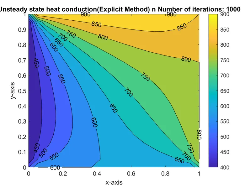
SNAP OF THE COMMAND WINDOW

So we conclude,

In Explicit, we cannot use the same time steps and length of mesh domain, as it yields to higher CFL number, which leads to unstable solution unconverging. For convenience, I have taken the time steps and length domain for both the x and y-axis mentioned in the code section. Iteration methods not required and results from both implicit and explicit methods are almost the same.

SNAP OF THE WORKSPACE

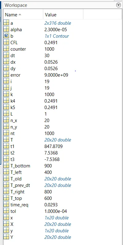
Solving Transient state 2D Heat Conduction IMPLICIT Method

MAIN PROGRAM

clear all 
close all
clc

% Inputs
L=1;
n_x = 20;
n_y = 20;
x = linspace(0,L,n_x);
y = linspace(0,L,n_y);
dx = x(2) - x(1);
dy = y(2) - y(1);
dt = 1e-2;
nt = 2000;
error = 9e9;
tol = 1e-4;

% boundary conditions
T_left = 400;
T_top = 600;
T_right = 800;
T_bottom = 900;
T = ones(n_x,n_y);

% Temperature at the boundary
T(2:n_y - 1,1) = T_left;
T(2:n_y - 1,n_x) = T_right;
T(1,2:n_x - 1) = T_top;
T(n_x,2:n_y - 1) = T_bottom;
 
T(1,1) = (T_top + T_left)/2;
T(n_x,n_y) = (T_right + T_bottom)/2;
T(1,n_y) = (T_top + T_right)/2;
T(n_x,1) = (T_left + T_bottom)/2;

alpha = 1;
k4 = (alpha*dt)/(dx^2);
k5 = (alpha*dt)/(dy^2);

jacobi_unsteady_imp(T,x,y,n_x,n_y,tol,k4,k5,nt)
 
gauss_unsteady_imp(T,x,y,n_x,n_y,tol,k4,k5,nt)
  
sor_unsteady_imp(T,x,y,n_x,n_y,tol,k4,k5,nt)

JACOBI-ITERATION

 %Jacobi Iteration implicit
function jacobi_unsteady_imp(T,x,y,n_x,n_y,tol,k4,k5,nt)
  [X,Y]=meshgrid(x,y);
   T_old = T;
   T_dt = T_old;
    
   t1 = (1 + 2*k4 + 2*k5)^(-1);
   t2 = k4*t1;
   t3 = k5*t1;  
   counter = 1;
   tic
      
   for k = 1:nt 
   error = 9e9;
   while(error>tol)  
      
    for i = 2:n_x - 1 
      for j = 2:n_y - 1
          H = (T_old(i - 1,j) + T_old(i + 1,j));
          V = (T_old(i,j - 1) + T_old(i,j + 1));
          T(i,j) = ((T_dt(i,j)*t1) + (H*t2) + (V*t3));
       end
     end
      error = max(max(abs(T_old - T)));
      T_old = T;
      counter = counter + 1;
    end
     T_dt = T;
    end
  time_req = toc;
  
  figure(1)
  contourf(x,y,T);
  [a b] = contourf(x,y,T);
  clabel(a,b);
  xlabel('x-axis');
  ylabel('y-axis');
  colorbar
  hold on;
  title_name = (sprintf('Plot for solving Transient state heat conduction equation implicitly using Jacobi method \n No. of iterations= %d \n',counter));
  title(title_name)
  file = (sprintf('2D Transient state heat conduct JacobiImplicit.png'));
  saveas(gca,file);
  fprintf('Number of iteration %d \n',counter);
  fprintf('Time taken for solving equation is %f \n',time_req);
end

GAUSS-ITERATION

% Gauss seidel
function gauss_unsteady_imp(T,x,y,n_x,n_y,tol,k4,k5,nt)
  
  t1 = (1 + (2*k4) + (2*k5))^(-1);
  t2 = k4*t1;
  t3 = k5*t1;
  T_old = T;
  T_dt = T_old;
  gauss_iteration = 1;
  tic
  
  for k = 1:nt 
    error = 9e9;
    while(error>tol)
  
    for i = 2:n_x - 1
      for j = 2:n_y - 1
      H = (T(i - 1,j) + T(i + 1,j));
      V = (T(i,j - 1) + T(i,j + 1));
      T(i,j) = ((T_dt(i,j)*t1) + (H*t2) + (V*t3));
      end
    end
    error=max(max(abs(T_old - T)));
    T_old = T;
    gauss_iteration = gauss_iteration + 1;
    end
   T_dt = T_old;
  end

time_req = toc;
figure(2)
[X,Y] = meshgrid(x,y);
[a b] = contourf(x,y,T);
clabel(a,b);
title_name = (sprintf('Plot for solving Transient state heat conduction equation implicitly by using gauss method \n No. of iterations: %d \n',gauss_iteration));
title(title_name)
xlabel('x-axis');
ylabel('y-axis');
colorbar
hold on;
file = sprintf('2D transient state heat conduction Gauss Siedel method IMLICITLY.png');
saveas(gca,file);
fprintf('Number of iteration %d \n',gauss_iteration);
fprintf('Time taken for solving equation is %f \n',time_req);
end

SOR-ITERATION

% SOR iteration
function sor_unsteady_imp(T,x,y,n_x,n_y,tol,k4,k5,nt)
  T_old = T;
  T_dt = T_old;
  
  % relaxation factor calculation
  z = cos(pi/n_x) + cos(pi/n_y);
  omega = 4/(2 + sqrt(4 - z^2));
  
  t1 = (1 + (2*k4) + (2*k5))^(-1);
  t2 = k4*t1;
  t3 = k5*t1;
  T_old = T;
  T_dt = T_old;
  sor_iteration = 1;
  tic
  for k = 1:nt    
   error = 9e9;
   while(error>tol) 
  
    for i = 2:n_x - 1
     for j = 2:n_y - 1
      H = (T(i - 1,j) + T(i + 1,j));
      V = (T(i,j - 1) + T(i,j + 1));
      T(i,j) = (omega*((T_dt(i,j)*t1) + (H*t2) + (V*t3)) - (omega - 1)*T_old(i,j));
     end
    end
    error = max(max(abs(T_old - T)));
    T_old = T;
    sor_iteration=sor_iteration+1;
   end
   T_dt = T;
  end

time_req = toc;
figure(3)
contourf(x,y,T);
[a b] = contourf(x,y,T);
clabel(a,b);
xlabel('x-axis');
ylabel('y-axis');
colorbar
hold on
title_name = (sprintf('Plot for solving Transient state heat conduction implicitly using SOR method \n No. of iterations: %d \n',sor_iteration));
title(title_name)
file = sprintf('2D Transient state heat conduction SOR method IMPLICITLY1.png');
saveas(gca,file);
fprintf('Relaxation factor considered is %f \n',omega);
fprintf('Number of iterations %d \n',sor_iteration);
fprintf('Time taken for solving equation is %f \n',time_req);
end

RESULTS

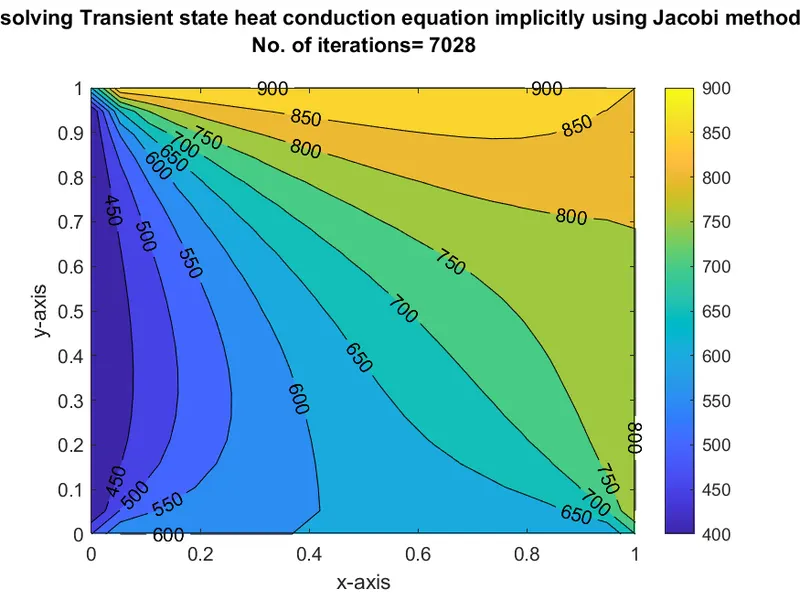
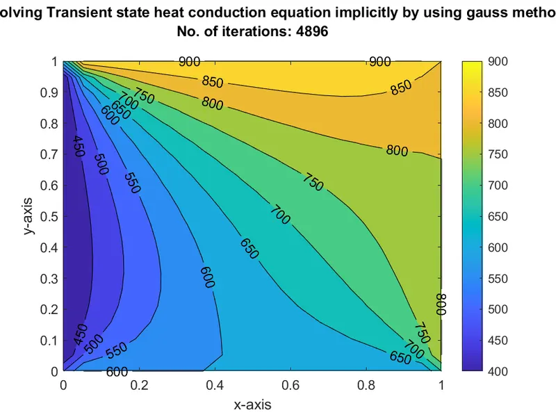
SNAP OF THE COMMAND WINDOW

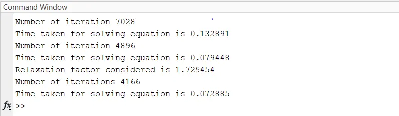
So we conclude,

Total no.of iteration is totally depends on dx,dy,dt,`alpha`,c1,c2,c values. Gauss method has a high convergence rate while comparing to the Jacobi method Gauss method and SOR method have the same convergence rate because we assume relaxation factor w=1.

SNAP OD THE WORKSPACE

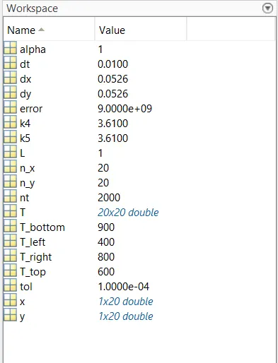
TOTAL CONCLUSION

The computational time and iteration required are SOR<GS<JACOBI for both steady and unsteady states. The implicit methods can be used to problems when converged results are needed in less computation time as they are unconditionally stable. With increases in time step size, the convergence rate is increased which leads to a steady-state with less no. of iterations. The explicit method results in time-accurate solutions as it is governed by stability criteria when not satisfied it leads to an unstable solution and requires more iterations to attain a steady-state. Explicit approach information from a given cell or mesh element must propagate to its immediate neighbors, hence the low CFL number needs to be considered.

Hence for this time step size, the explicit scheme leads to a faster convergent rate and as the time step size is small the number of iterations increases for the implicit scheme which results in slower convergence rate.