Week 5.1 - Mid term project - Solving the steady and unsteady 2D heat conduction problem
Aim: To solve steady and unsteady 2d heat conduction equations in Matlab using iterative techniques like jocobi, gauss-siedal, sor(successive over-relaxation)
Objective: To solve 2d heat conduction equation with the given boundary condition and to implement the iterative techniques
and to compare the results and to use both implicit and explicit solvers for the transient state.
Theory:
`(delT)/(delt)=alpha((del^2t)/(delx^2)+(del^2t)/(dely^2)+(del^2t)/(delz^2))`
this is a 3-d heat conduction equation in this equation `(delT)/(delt)` implies the change of temperature with respect to time and `alpha` is diffusivity this determines how fast the temperature is spreading throughout the material. and `(del^2t)/(delx^2)+(del^2t)/(dely^2)+(del^2t)/(delz^2)` this is change of temperature with respect to space.
in this problem, we will deal with the 2D heat conduction equation.
Boundary conditions :
the given boundary conditions are
Top Boundary = 600 K
Bottom Boundary = 900 K
Left Boundary = 400 K
Right Boundary = 800 K
so the left top corner will have a temperature (600+400)/2=500 k
the top right corner will have a temperature (800+600)/2=700 k
the bottom left corner will have a temperature (900+400)/2=650 k
the bottom right corner will have a temperature (900+800)/2=850 k
Matlab code:
in this program, there will be the main function in which the boundary condition, tolerance, alpha, time step, mesh domain, total simulation time, number of time steps, and CFL number will be defined and will call the necessary function to solve the 2D heat conduction equation by various iterative techniques
Main code
close all
clear all
clc
%soving 2D steady heat conduction equation
nx=101;
ny=nx;%nx and ny is number of grid points in x and y direction
x=linspace(0,1,nx);
y=linspace(0,1,ny);
dt=0.1;
t=300;
nt=t/dt;
dx=x(2)-x(1);%distance between the grid points along x direction
dy=y(2)-y(1);
alpha=1.75e-4;
%ablsoute error criteria and tolrence
%defining boundary condition
T=300*ones(nx,ny);
T(:,1)=400;
T(:,end)=800;
T(1,:)=600;
T(end,:)=900;
%defifning the temperature at corner points
T(1,1)=(400+600)/2;%top left corner
T(nx,1)=(900+400)/2;%bottom left corner
T(nx,ny)=(900+800)/2;%bottom right corner
T(1,ny)=(600+800)/2;%top right corner
t_prev=T;
t_old=T;
%term k in the discritized heat conduction equation 2D
k=2*((dx^2 + dy^2)/((dx^2)*(dy^2)));
k1=alpha*dt/dx^2;
k2=alpha*dt/dy^2;
cfl=k1+k2;
%diefing a variable t_old for refernce to iterate
%this is temprature at previous time step . this variable will be used in transiet implicit solvers

%jocobi_iterexplicit(nx,ny,t_old,dx,dy,T,k,x,y);
%gauss_seidalexplicit(nx,ny,t_old,dx,dy,T,k,x,y);
%sor_gs(nx,ny,t_old,dx,dy,T,k,x,y);
%transient_expilcit(nx,ny,t_old,dx,dy,T,x,y,cfl,nt,dt,t,alpha);
%transient_jociboi_implicit(nx,ny,t_old,T,x,y,nt,t,t_prev,alpha,dx,dy,dt);
%transient_gauss_siedal_implicit(nx,ny,t_old,T,x,y,nt,t,t_prev,alpha,dx,dy,dt,k1,k2);
%transient_sor_gauss(nx,ny,t_old,T,x,y,nt,t,t_prev,alpha,dx,dy,dt,k1,k2);
Steady-state 2D heat conduction in explicit form :
`(T^(n+1) -T^(n))/dt=alpha((T_(i+1,j)-2T_(i,j)+T_(i-1,j))/dx^2+(T_(i,j+1)-2T_(i,j)+T_(i,j-1))/dy^2)`
here the time derivative in the heat equation is in second-order Taylor approximation form and the spatial derivatives in the 2d heat conduction equation are approximated in second-order central differentiation. and this polynomial equation will be used to solve the 2d heat conduction equation with the given boundary condition with different iterative methods.
Steady-state 2d heat conduction equation in the explicit form:
since it is a steady-state the time derivative term will not be present in the equation so the solution is only dependent on the spatial derivative term so the discretized 2d heat conduction equation will become as `(T_(i+1,j)-2T_(i,j)+T_(i-1,j))/dx^2+(T_(i,j+1)-2T_(i,j)+T_(i,j-1))/dy^2=0`
to make things simple let's say that the current nodal point is T_P, and by keeping the current nodal point as a reference the left nodal point be T_L likewise the corresponding right, top, bottom nodal point are referred to as T_R, T_T, T_B respectively
so the equation becomes `2T_p/dx^2 +2T_p/dy^2=(T_L+T_R)/dx^2+(T_T+T_B)/dy^2`
`T_p=((T_L+T_R)/dx^2+(T_T+T_B)/dy^2)/k` where `K=2(dx^2+dy^2)/(dx^2dy^2)`
this equation is solved in 3 iterative methods namely jocobi,gauss-seidel, SOR.
Matlab function of the steady-state 2-D heat conduction equation by jocobi method:
function out=jocobi_iterexplicit(nx,ny,t_old,dx,dy,T,k,x,y)
%function for jocobi method

iter=0;
error=1;
tol=1e-4;
while (error>tol)

    for i=2:nx-1
        for j=2:ny-1
            term1=((t_old(i-1,j)+t_old(i+1,j))/dx^2);
            term2=((t_old(i,j-1)+t_old(i,j+1))/dy^2);
            T(i,j)=(term1+term2)/k;
        end
    end
    error=max(max((abs(t_old-T))));
    t_old=T;
    iter=iter+1;
end
disp (error)
figure (1)
[u,v]=contourf(x,y,T);
clabel(u,v);
colorbar;
colormap (jet)
ax=gca;
ax.YDir='reverse';
xlabel('Xaxis')
ylabel('yaxis')
title({'steady state temperature profile';['iteration method=jocobi explicit method'];['nmber of iterration=',num2str(iter)];})
grid on
end
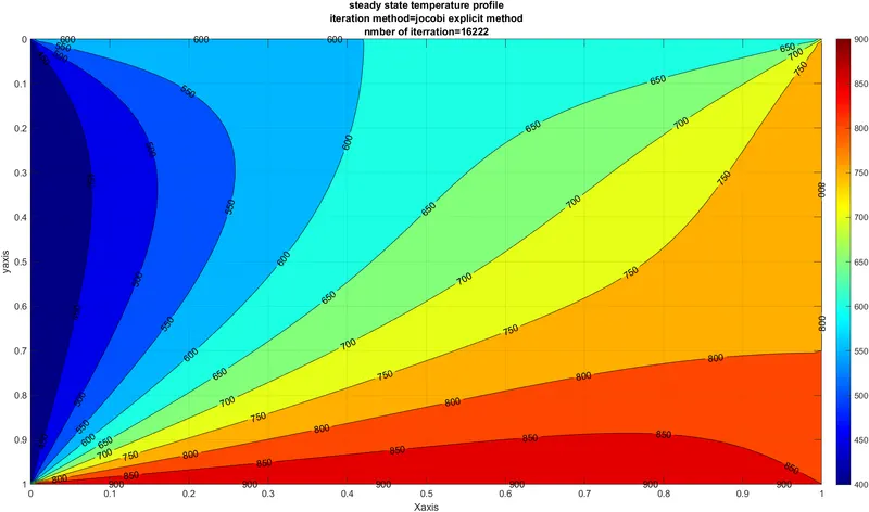
Steady-state temperature profile by jocobi method:
Matlab function of the steady-state 2-D heat conduction equation by gauss seidel method:
function out1=gauss_seidalexplicit(nx,ny,t_old,dx,dy,T,k,x,y)
%function for gauss seidal explicit method
iter=0;
tol=1e-4;
error=1;
while (error>tol)
    for i=2:nx-1
        for j=2:ny-1
            term1=((T(i-1,j)+t_old(i+1,j))/dx^2);
            term2=((T(i,j-1)+t_old(i,j+1))/dy^2);
            T(i,j)=1/k*(term1+term2);
        end
    end
    error=max(max((abs(t_old-T))));
    t_old=T;
    iter=iter+1;
end
disp (error)
figure (2)
[u,v]=contourf(x,y,T);
clabel(u,v);
colorbar;
colormap (jet)
ax=gca;
ax.YDir='reverse';
xlabel('Xaxis')
ylabel('yaxis')
title({'steady state temperature profile';['iteration method=gauss seidal explicit method'];['nmber of iterration=',num2str(iter)];})
grid on
end
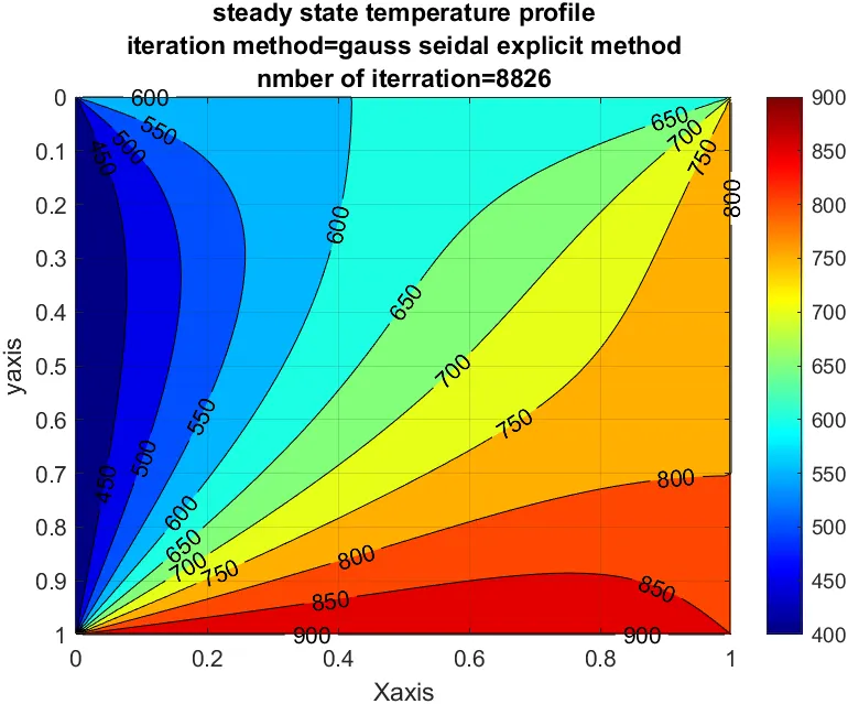
Steady-state temperature profile by the gauss-seidel method:
Matlab function of the steady-state 2-D heat conduction equation by SOR method:
function out2=sor_gs(nx,ny,t_old,dx,dy,T,k,x,y)
%function for gauss seidal explicit method
iter=0;
error=1;
tol=1e-4;
omega=1.6;
while (error>tol)
    for i=2:nx-1
        for j=2:ny-1
            term1=((T(i-1,j)+t_old(i+1,j))/dx^2);
            term2=((T(i,j-1)+t_old(i,j+1))/dy^2);
            T_gs=1/k*(term1+term2);
            T(i,j)=(1-omega)*(t_old(i,j))+T_gs*(omega);
        end
    end
    error=max(max((abs(t_old-T))));
    t_old=T;
    iter=iter+1;
end
disp (error)
figure (2)
[u,v]=contourf(x,y,T);
clabel(u,v);
colorbar;
colormap (jet)
ax=gca;
ax.YDir='reverse';
xlabel('Xaxis')
ylabel('yaxis')
title({'steady state temperature profile';['iteration method=SOR(gauss seidel)'];['nmber of iterration=',num2str(iter)];})
grid on
end
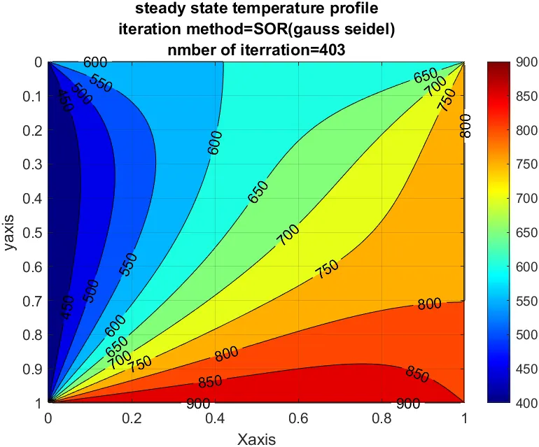
Steady-state temperature profile by the SOR method:
Discussion on the solution of steady-state 2-D heat conduction equation by various iterative methods:
| iterative methods | jocobi method | gauss-seidel method | SOR method(`omega` as 1.96) |
| number of iterations | 16222 | 8826 | 593 |
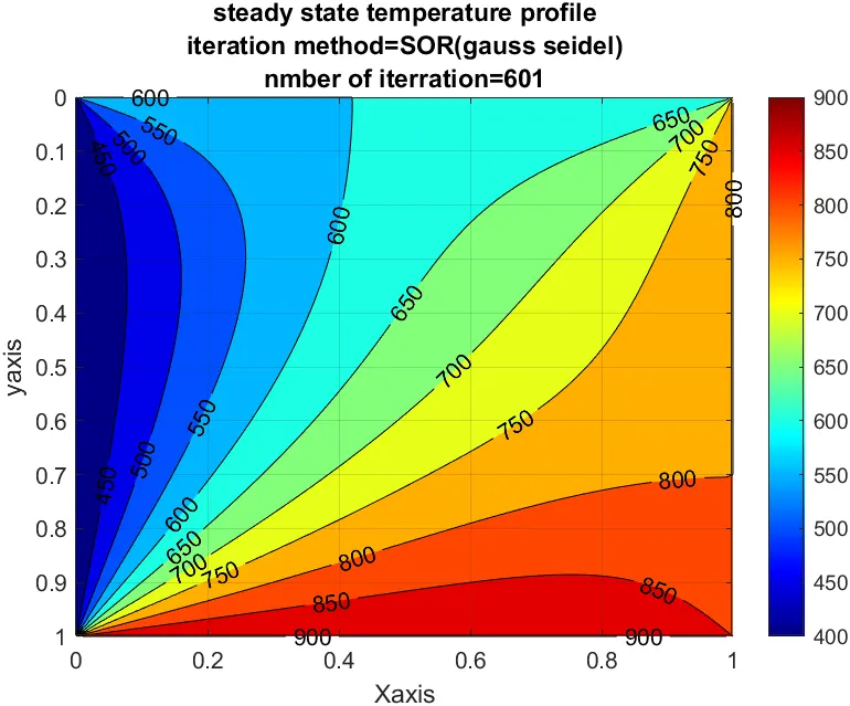
As we can see the above profile we can say that the total number of iteration is less in the SOR method compared to jocobi, and gauss seidel methods and w can also observe that the jocobi method needs more number iteration compared to gauss-seidel methods this is because in jocobi method we are giving an initial value and from that, we will be getting a new value. and for calculating the next value we will be using the old value that has calculated in the previous iteration. but in the gauss seidel method, we are calculating our initial value by the given initial condition but for the next iteration, we are using the new value that has been calculated for the previous node in the same iteration so we can able to converge with less iteration compared to jocobi method. in the SOR method, we are using the relaxation factor `omega` known as omega which will help us to converge faster but the relaxation factor should be chosen carefully because a wrong relaxation factor can lead to oscillating between the converging solution which may increase the number of iteration
for example, the below plot is the profile of the 2-d heat conduction equation but with an `omega` value of 1.97, as we can see the number of iteration is increased means that the simulation time will increase.
Transient state 2-D Heat conduction equation:
In this condition, the change in temperature with respect to time is also taken as a part of the solution.the discretized equation of this transient state heat conduction equation is
`(T_p)^(n+1)=(T_p)^n+alpha dt((T_R-2T_P+T_L)/dx^2+(T_T-2T_P+T_B)/dy^2)^n` this is in explicit form
`(T_p)^(n+1)=(T_p)^n+alpha dt((T_R-2T_P+T_L)/dx^2+(T_T-2T_P+T_B)/dy^2)^(n+1)` this is in implicit form
note : here n+1 and n represents the time steps it is not the power of that equation.
in the explicit form, we know the terms that are present in the RHS but in implicit we don't know some of the terms because it is present in the next time step that is yet to is calculated using the same equation.
in simple words, we can say that in the explicit method for 1 iteration we will be marching through the entire domain one time.
and in the explicit method, we will be marching through space so many times till the solution converges or the solution is below the tolerance level in a single time step.
and a number of time steps can be calculated by the total number of time steps =total simulation time * time step.
the implicit form of the equation can be solved by matrix manipulation but it is a bit hard since the no. of the equation is more so we will use iterative methods
so the implicit method can be written as
`(T_p)^(n+1)=((T_p)^(n)+k1(T_L)^(n+1)+k1(T_R)^(n+1)+k2(T_T)^(n+1)+k2(T_B)^(n+1))/(1+2k1+2k2)`
where the k1=`alpha(dt/dx^2)` , k2=`alpha(dt/dy^2)` which is a part the discretized equation.
note: here n+1 and n represent the time steps it is not the power of that equation.
and here the `alpha` is assumed to be 1.75e-4 for all methods.
Matlab function Transient state equation by the explicit method :
function out4=transient_expilcit(nx,ny,t_old,dx,dy,T,x,y,cfl,nt,dt,t,alpha)
iter=0;
tol=1e-4;
cfl;
%time loop for transwint conditon
for g=1:nt
    for i=2:nx-1 %space loop for x
        for j=2:ny-1 %space loop for y
            term1=alpha*dt*(t_old(i+1,j)-2*t_old(i,j)+t_old(i-1,j))/dx^2;
            term2=alpha*dt*(t_old(i,j+1)-2*t_old(i,j)+t_old(i,j-1))/dy^2;
            T(i,j)=t_old(i,j)+(term1+term2);

        end
    end
    t_old=T;
    iter=iter+1;
end
disp (iter)
figure (2)
[u,v]=contourf(x,y,T);
clabel(u,v);
colorbar;
colormap (jet)
ax=gca;
ax.YDir='reverse';
xlabel('Xaxis')
ylabel('yaxis')
title({'steady state temperature profile';['iteration method = transient explicit'];[' nmber of iterration= ',num2str(iter),' time= ',num2str(t),' s ',' CFL = ',num2str(cfl)];})
grid on

end
Transient-state temperature profile by the explicit method:
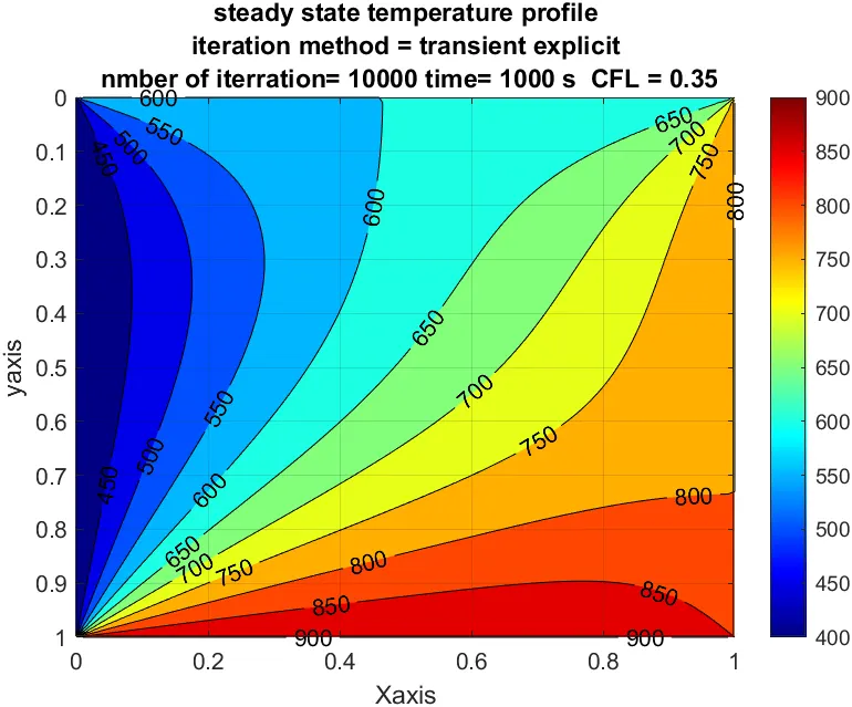
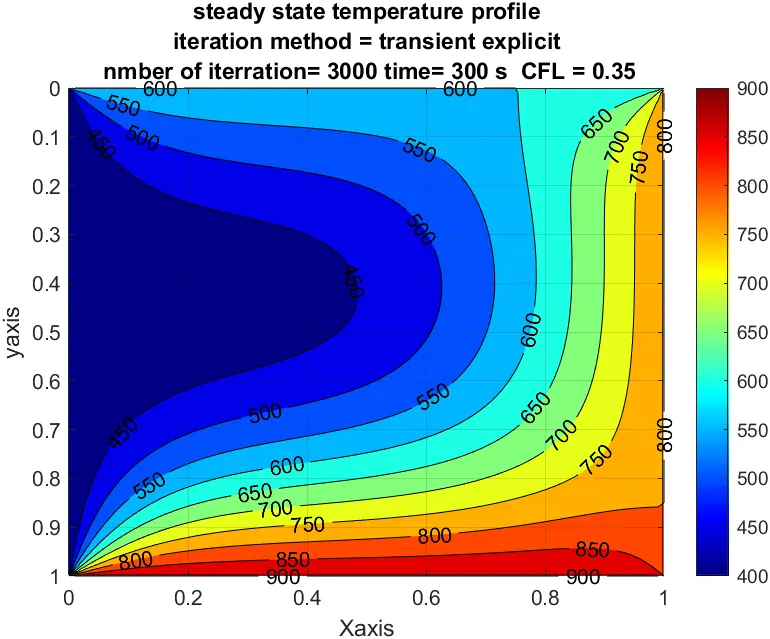
in the above plot, simulation time is varied means at 300s for the same time step steady state is not achieved. steady-state is achieved at t=1000 s, and the alpha value for this simulation is 1.47e-4
Observation in the transient state in the explicit method
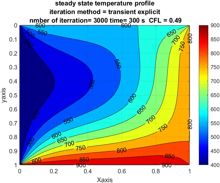
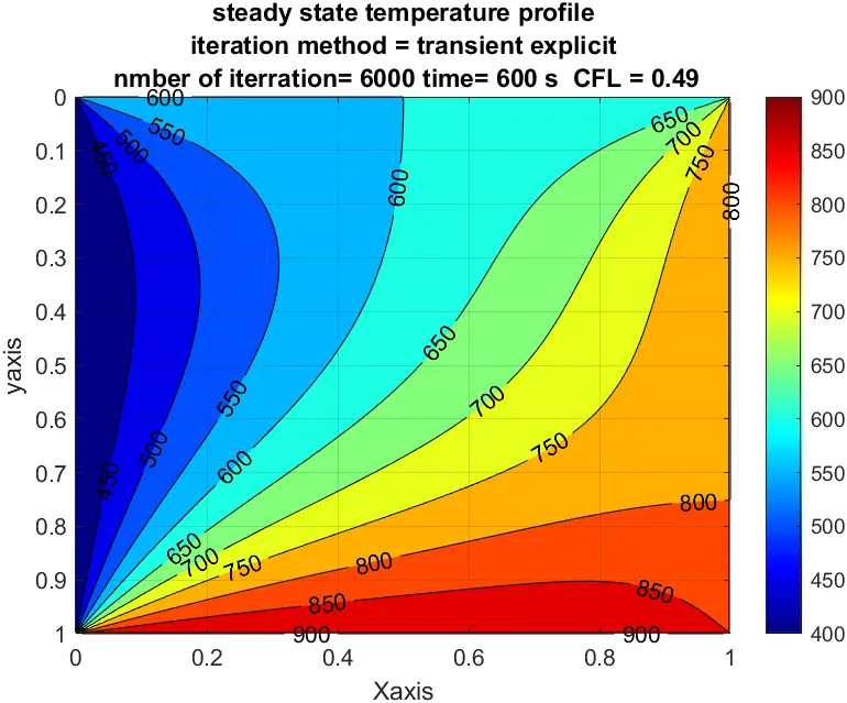
By comparing the plots from the previous session we can able to tell that even for the same simulation time (t=300s) the convergence of the solution Is a bit faster when the CFL number is higher. and we can also say that the steady-state is achieved by simulating for 600s so the CFL number also plays a major role while using explicit. we need to note that the alpha value for this plot is `2.45e-4`so the CFL number is changed which is making our simulation a bit faster.
Transient state heat conduction equation by the implicit method :
Matlab function for transient state heat conduction equation by jocobi method :
function out4=transient_jociboi_implicit(nx,ny,t_old,T,x,y,nt,t,t_prev,alpha,dx,dy,dt)
iter=0;
tol=1e-4;
k1=alpha*dt/(dx^2);
k2=alpha*dt/(dy^2);
cfl=k1+k2;
for g=1:nt %time loop for every time step we will itarate in the space till the solution converge
    error=1;
    while (error>tol)%space loop
        for i=2:nx-1
            for j=2:ny-1
                H=t_old(i-1,j)+t_old(i+1,j);
                v=t_old(i,j-1)+t_old(i,j+1);
                term1=1/(1+(2*k1)+(2*k2));
                T(i,j)=(t_prev(i,j)*term1)+(term1*k1*H)+(term1*k2*v);
            end
        end
        error=max(max(abs(t_old-T)));
        iter=iter+1;
        t_old=T;

    end
    t_prev=T;

end
disp (iter)
[u,v]=contourf(x,y,T);
clabel(u,v);
colorbar;
colormap (jet)
ax=gca;
ax.YDir='reverse';
xlabel('Xaxis')
ylabel('yaxis')
title({'steady state temperature profile';['transient jocobi iteration method'];['nmber of iterration=',num2str(iter)];})
grid on
end
Matlab function for transient state heat conduction equation by the gauss-seidel method :
function out5=transient_gauss_siedal_implicit(nx,ny,t_old,T,x,y,nt,t,t_prev,alpha,dx,dy,dt,k1,k2)
iter=0;
tol=1e-4;
for g=1:nt %time loop for every time step we will itarate in the space till the solution converge
    error=1;
    while (error>tol)%space loop
        for i=2:nx-1
            for j=2:ny-1
                H=T(i-1,j)+t_old(i+1,j);
                v=T(i,j-1)+t_old(i,j+1);
                term1=1/(1+(2*k1)+(2*k2));
                T(i,j)=(t_prev(i,j)*term1)+(term1*k1*H)+(term1*k2*v);
            end
        end
         error=max(max(abs(t_old-T)));
        iter=iter+1;
        t_old=T;

    end
    t_prev=T;

end
disp (iter)
[u,v]=contourf(x,y,T);
clabel(u,v);
colorbar;
colormap (jet)
ax=gca;
ax.YDir='reverse';
xlabel('Xaxis')
ylabel('yaxis')
title({'steady state temperature profile';['transient gauss seidal iteration method'];['nmber of iterration=',num2str(iter)];})
grid on
end
Matlab function for transient state heat conduction equation by the SOR method :
function out6= transient_sor_gauss(nx,ny,t_old,T,x,y,nt,t,t_prev,alpha,dx,dy,dt,k1,k2)
iter=0;
tol=1e-4;
k1=alpha*dt/(dx^2);
k2=alpha*dt/(dy^2);
cfl=k1+k2;
omega=1.2;
for g=1:nt %time loop for every time step we will itarate in the space till the solution converge
    error=1;
    while (error>tol)%space loop
        for i=2:nx-1
            for j=2:ny-1
                H=T(i-1,j)+t_old(i+1,j);
                v=T(i,j-1)+t_old(i,j+1);
                term1=1/(1+(2*k1)+(2*k2));
                T(i,j)=(t_prev(i,j)*term1)+(term1*k1*H)+(term1*k2*v);%this is gauss seidal technique
                T(i,j)=(1-omega)*(t_old(i,j))+T(i,j)*(omega);;%applying gauss seiald in sor method in order to reduce the number of iteration
            end
        end
        error=max(max(abs(t_old-T)));
        iter=iter+1;
        t_old=T;

    end
    t_prev=T;

end
disp (iter)
[u,v]=contourf(x,y,T);
clabel(u,v);
colorbar;
colormap (jet)
ax=gca;
ax.YDir='reverse';
xlabel('Xaxis')
ylabel('yaxis')
title({'steady state temperature profile';['transient state by SOR iteration method'];['nmber of iterration=',num2str(iter)];})
grid on
end
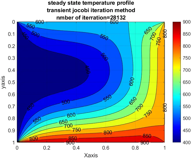
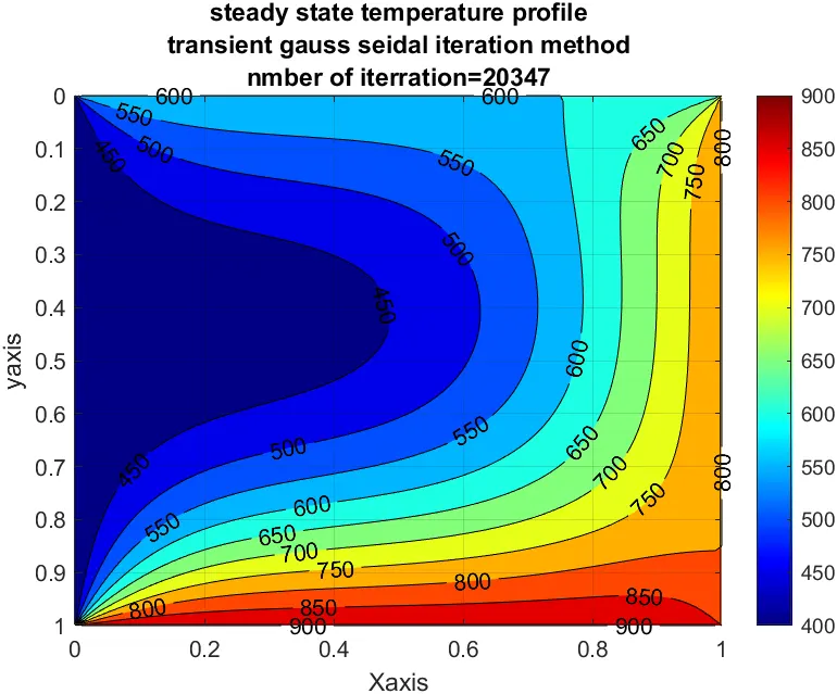
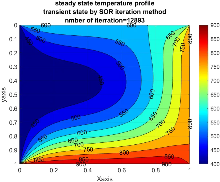
Profile of the temperature distribution of jocobi, gauss seidel, SOR method :
this simulation time for all the iterative methods is set to be 300s and `alpha` 1.75e-4
Observation:
the number of iteration for the same simulation time is the no of iterations different.
| iterative method | jocobi | gauss seidel | SOR |
| number of iteration | 28132 | 20347 | 12893 |
By this table we can say that the number of iteration is less is SOR compared to the other two, and the number of iteration is less in gauss seidel compared to jocobi for the same simulation time. and the omega value in the SOR method is 1.2 with which we can able get an optimized number of iteration.