Week 3.5 - Deriving 4th order approximation of a 2nd order derivative using Taylor Table method

Deriving a fourth-order approximation of second-order derivative using central difference scheme, right-skewed, left-skewed method:

1)Using the central difference method

The central difference scheme basically gets the information from a neighboring node from both sides by taking a reference node.

we will use the Taylor method of approximation to approximate.

the number of nodes to be selected is given by,

the no. of nodes=order of the approximation + order of the derivative -1, that is n=p+q-1.

so here n=4+2-1=5, so we need 5 nodes to get a good approximated value

so the function that to be approximated is `f(x)=exp(x)*cos(x)`

the analytical derivative of second-order of the above function is `(del^2f(x))/(delx)=-2exp(x)sin(x)`

the numerical solution by central difference method is

`f''(x)~~(a*f(x-2dx)+b*f(x-dx)+c*f(x)+d*f(x+1)+e*f(x+2dx))/dx^2`

here a,b,c,d,e are the coefficients that make the other higher-order derivtes terms(HOD) zero and the term f(x) and first order deritve of the function also zero so we can able to approximate the second order derivative of the function by using talyor table method

[note: the coefficients are calculated by expanding and manipulation of the equation in order to get the desired equation that will solve for the fourth-order approximation of second-order derivative here I am not going to show the manipulation of the numerical equation]

talyor table for fourth order approximation of second order derivative using central difference method

`dx^2*f''(x)`	f(x)	dx*f'(x)	dx^2*f''(x)	dx^3*f'''(x)	dx^4*f''''(x)	dx^5*f'''''(x)	dx^6*f''''''(x)
`af(x-2dx)`	a	-2a	`4(a)/2`	`-8/6a`	`16/24a`	`-32/120a`	`64/240a`
`cf(x)`	c	0	0	0	0	0	0
`d*f(x+dx)`	d	d	`d/2`	`d/6`	`d/24`	`d/120`	`d/240`
`e*f(x+2dx)`	e	2e	`4/2e`	`8/6e`	`16/24e`	`32/120e`	`64/240e`
`b*f(x-dx)`	b	-b	`b/2`	`-b/6`	`b/24`	`-b/120`	`b/240`
summation	0	0	1	0	0	~	~

after solving the equation we will get a system of equations corresponding to the coefficient

`a+b+c+d+e=0`

`-2a-b+d+2e=0`

`2a +(b)/2+(d)/2+2e=1`

`-(8)/6a-(b)/6+d/6+e(8)/6=0`

`16a+b+d+16e=0`

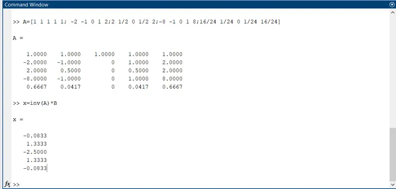
we can solve for a,b,c,d,e by using matrix

`[[1,1,1,1,1],[-2,-1,0,1,2],[2,1/2,0,1/2,2],[-8,-1,0,1,8],[16,1,0,1,16]]*[[a],[b],[c],[d],[e]]=[[0],[0],[1],[0],[0]]`

by solving above equation,a=-0.0833,b=1.3333,c=2.5000,d=1.3333,e=-0.0833

2)Using right sided sekwed method:

the right sided skewed method takes the information form right side only it doest care about left side information it will approximate the function by taking required number of nodes, the number nodes required for this method is given by a formula `n=p + q` where p is order of approximation and q is the order of the derivative of the function.

n=4+2=6 , in this method we need 6 nodes to get an fourth order approximation of second order derivative.

the numerical solution for fourth order approximation and second order derivative is

`f''(x)~~(af(x)+bf(x+dx)+cf(x+2dx)+df(x+3dx)+ef(x+4dx)+gf(x+5dx))/dx^2`

here a,b,c,d,e are the coefficients that make the other higher-order derivtes(HOD) zero and the term f(x) and first order deritve of the function also zero so we can able to approximate the second order derivative of the function by using talyor table method

[note: the coefficients are calculated by expanding and manipulation of the equation in order to get the desired equation that will solve for the fourth-order approximation of second-order derivative here I am not going to show the manipulation of the numerical equation]

talyor table for fourth order approximation of second order derivative using right sided sekwed difference method

`dx^2*f''(x)`	f(x)	dx*f'(x)	dx^2*f''(x)	dx^3*f'''(x)	dx^4*f''''(x)	dx^5*f'''''(x)
`af(x)`	a	0	0	0	0	0
`cf(x+2dx)`	c	2c	`4/2c`	`8/6c`	`16/24c`	`32/120c`
`d*f(x+3dx)`	d	3d	`9/2d`	`27d/6`	`d81/24`	`d243/120`
`e*f(x+4dx)`	e	4e	`16/2e`	`64/6e`	`256/24e`	`1024/120e`
`b*f(x+dx)`	b	b	`b/2`	`b/6`	`b/24`	`b/120`
`gf(x+5dx)`	g	5g	`25/2g`	`125/6g`	`625/24g`	`3125/120g`
summation	0	0	1	0	0	0

so we get an system of equation

`a+b+c+d+e+g=0`

`b+2c+3d+4e+5g=0=0`

`(b)/2+4/2c+d9/2+8e+g25/2=1`

`(b)/6+d8/6+27/6d+e(64)/6+g125/6=0`

`b1/24+16/24c+d81/24+256/24e+625/24g=0`

`1/120b+32/120c+243/120d+1024/120e+3125/120g=0`

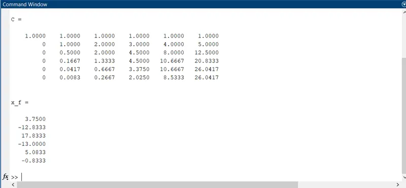
we can solve for a,b,c,d,e by using matrix

`[[1,1,1,1,1,1],[0,1,2,3,4,5],[0,1/2,4/2,9/2,8,25/2],[0,1/6,8/6,27/6,64/6,125/6],[0,1/24,16/24,81/24,256/24,625/24],[0,1/120,32/120,243/120,1024/120,3125/120]]*[[a],[b],[c],[d],[e],[g]]=[[0],[0],[1],[0],[0],[0]]`

by solving above equation we get

a=3.7500,b=-12.8333,c=17.8333,d=-13.0000,e=5.0833,g=-0.8333

3)Using left-sided skewed method:

the left-sided skewed method takes the information from the left side only it doest care about right side information it will approximate the function by taking the required number of nodes, the number nodes required for this method is given by a formula `n=p + q` where p is the order of approximation and q is the order of the derivative of the function.

n=4+2=6, in this method we need 6 nodes to get a fourth-order approximation of second-order derivative.

the numerical solution for fourth-order approximation and second-order derivative is

`f''(x)~~(af(x-5dx)+bf(x-4dx)+cf(x-3dx)+df(x-2dx)+ef(x-dx)+gf(x))/dx^2`

here a,b,c,d,e are the coefficients that make the other higher-order derivatives(HOD) zero, and the term f(x) and first-order derivative of the function also zero so we can able to approximate the second-order derivative of the function by using Taylor table method

[note: the coefficients are calculated by expanding and manipulation of the equation in order to get the desired equation that will solve for the fourth-order approximation of second-order derivative here I am not going to show the manipulation of the numerical equation]

Taylor table for fourth-order approximation of second order derivative using right sided sekwed difference method

`dx^2*f''(x)`	f(x)	dx*f'(x)	dx^2*f''(x)	dx^3*f'''(x)	dx^4*f''''(x)	dx^5*f'''''(x)
`af(x-5dx)`	a	-5a	`25/2a`	`-125/6a`	`625/24`	`-3125/120a`
`fc(x-3dx)`	c	-3c	`9/2c`	`-27/6c`	`81/24c`	`-243/120c`
`d*f(x-2dx)`	d	-2d	`4/2d`	`-8d/6`	`d16/24`	`-32/120d`
`e*f(x-dx)`	e	-e	`e/2`	`-e/6`	`e/24`	`-e/120`
`b*f(x-4dx)`	b	-4b	`b16/2`	`-64/6b`	`256/24b`	`-b1024/120`
`gf(x)`	g	0	`0`	`0`	`0`	`0`
summation	0	0	1	0	0	0

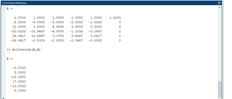
by solving the above equation using matrix we get

a=-0.8333,b=5.0833,c=-13.0000,d=19.8333,e=-12.8333,g=3.75000

Matlab program:

clear all
close all
clc

%the point where the function is evaluated
x=pi/3;
dx=linspace(pi/4,pi/400,50);

%a loop to get all dx values and pass it to the function
for i=1:length(dx)
   error=tlayor_table(x,dx(i));
   error_central_diff(i)=error(1);
   error_forwaed_diff(i)=error(2);
   error_backward_diff(i)=error(3);  
end
loglog(dx,error_central_diff,'r','marker','o')
hold on
loglog(dx,error_forwaed_diff,'g','marker','o')
loglog(dx,error_backward_diff,'b','marker','o')
xlabel('rage of dx')
ylabel('truncation error')
legend('central differnce','skewed right side differnce','skewed lift side differnce')
    

function tlayor_table:

function out= tlayor_table(x,dx)

%function to approximated f(x)=exp(x)*cos(x)
% the seconder order derivative of the function f''(x)=-2exp(x)sin(x)
analytical_derivative=-2*exp(x)*sin(x);


%calculating the coeffients in central differnce method
A=[1 1 1 1 1;-2 -1 0 1 2;2 1/2 0 1/2 2;-8 -1 0 1 8;16 1 0 1 16];
B=[0; 0;1;0;0];
%the below 5x1 martix contains the coefficent in the central differnce
x_c=linsolve(A,B);
%calculating the coeffients in right hand sekwed
C=[1 1 1 1 1 1;0 1 2 3 4 5;0 1/2 4/2 9/2 8 25/2;0 1/6 8/6 27/6 64/6 125/6;0 1/24 16/24 81/24 256/24 625/24;0 1/120 32/120 243/120 1024/120 3125/120];
D=[0;0;1;0;0;0];
%the below 6x1 martix contains the coefficent in the forward skewed method
x_f=linsolve(C,D);
%calculating the coeffients in left hand sekwed
E=[1 1 1 1 1 1;-5 -4 -3 -2 -1 0;25/2 16/2 9/2 4/2 1/2 0;-125/6 -64/6 -27/6 -8/6 -1/6 0;625/24 256/24 81/34 16/24 1/24 0;-3125/120 -1024/120 -243/120 -32/120 -1/120 0];
F=[0;0;1;0;0;0];
%%the below 6x1 martix contains the coefficent in the backward skewed method
x_b=linsolve(E,F);
%now applying the tlyor table we found the fourth order approximaton of second order derivative
%using central differnce scheme 
central_diff=(x_c(1)*exp(x-2*dx)*cos(x-2*dx)+x_c(2)*(exp(x-dx)*cos(x-dx))+x_c(3)*(exp(x)*cos(x))+x_c(4)*(exp(x+dx)*cos(x+dx))+x_c(5)*(exp(x+2*dx)*cos(x+2*dx)))/(dx^2);
%using forward skewed differnce method
forward_diff=(x_f(1)*(exp(x)*cos(x))+x_f(2)*(exp(x+dx)*cos(x+dx))+x_f(3)*(exp(x+2*dx)*cos(x+2*dx))+x_f(4)*(exp(x+3*dx)*cos(x+3*dx))+x_f(5)*(exp(x+4*dx)*cos(x+4*dx))+x_f(6)*(exp(x+5*dx)*cos(x+5*dx)))/(dx^2);
%using bacward skewed differnce method
backward_diff=(x_b(1)*(exp(x-5*dx)*cos(x-5*dx))+x_b(2)*(exp(x-4*dx)*cos(x-4*dx))+x_b(3)*(exp(x-3*dx)*cos(x-3*dx))+x_b(4)*(exp(x-2*dx)*cos(x-2*dx))+x_b(5)*(exp(x-dx)*cos(x-dx))+x_b(6)*(exp(x)*cos(x)))/(dx^2);

%now we are going to calculate the error values
%error of central differnce method
error_central=abs(analytical_derivative-central_diff);
%error of forward differnce method
error_forward=abs(analytical_derivative-forward_diff);
%error of backward differnce method
error_backward=abs(analytical_derivative-backward_diff);
%now we are going to store this error values in differnt variable
out(1)=error_central;
out(2)=error_forward;
out(3)=error_backward;
end

Graph comparing error from central,right-sided skewed,left-sided skewed methods:

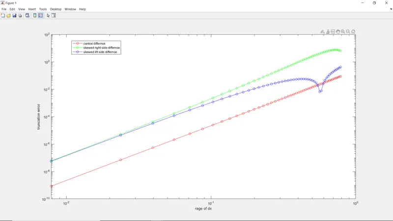
proof that the skewed scheme are fourth-order accurate

number of nodes in the stencil =6

order of derivative of the function=2

order of skewed scheme =number of nodes in stencil - order of derivative of the function that is approximated =6-2=4

so the order of skewed scheme is 4 that is it is a fourth-order approximation.

why a skewed scheme is useful?

in some complex problems, the numerical stencil will not be in a symmetric way for that type of problem we need skewed methods

What can a skewed scheme do that a CD scheme cannot?

in the boundary of a mesh, there won't be any node on the other side so we can only get the information from one side so a skewed scheme is used in this type of problem since we cannot able to take information from one of the sides of the node so we cannot use central scheme here

conclusion:

As we see in the above graph all the approximations are fourth-order but the central difference scheme has less error compared to other schemes because it gets the information from both sides of a node.