Week 11 - Simulation of Flow through a pipe in OpenFoam
Objective:
need to simulate an axis-symmetric flow through the pipe by applying wedge boundary condition the flow is laminar and flows through a constant cross-section pipe at an inlet Reynolds number of 2100 validate our results with Hagen-poiseullies equation
- Validate Hydro-dynamic length with the numerical result
- Validate the fully developed flow velocity profile with its analytical profile
- Validate maximum velocity and pressure drop for fully developed flow
- Post-process Shear stress and validate wall shear stress for fully developed flow
note: In this project, we have assumed some data.
Flow-through pipe :
This is one of the standard engineering flow we come across in our daily life. the flow in a pipe can be easily studied compared to other complex geometries and the flow can be laminar or turbulent. and this is determined by various factors like surface roughness, flow velocity, fluid property, pipe diameter because all of this affects a dimensionless number known as Reynolds number which is generally used to determine the type of flow(laminar or turbulent). and Reynolds number is the ratio between viscous force and inertial force
`Re=(v_(avg)*D)/nu`
Re<2300 is laminar flow
2300<Re<4000 is a transitional flow
Re>4000 turbulent flow
for laminar flow, there is a relation called the Hagen-poiseullies relation
`v_(avg)*A_c=(/_\p*pi*D^4)/(128muL)` where v_avg is the average velocity and Ac is an area of cross-section, L is the length of the pipe D is the diameter of the pipe. `/_\ p` is a pressure drop along the pipe.
Solution:
In this project, we assume our average velocity of the fluid as 0.16821 m/s, and by given Reynolds number our characteristic length that is the diameter in case of circular pipe is said to be D=0.019m so by the formula `L_e=0.05*Re*D`and the wedge angle will be 3 degrees we cay say that our hydrodynamic length will be 2m approximate so let us assume that our pipe length will be 3 meters approx and for the fluid properties lets consider water at 35C
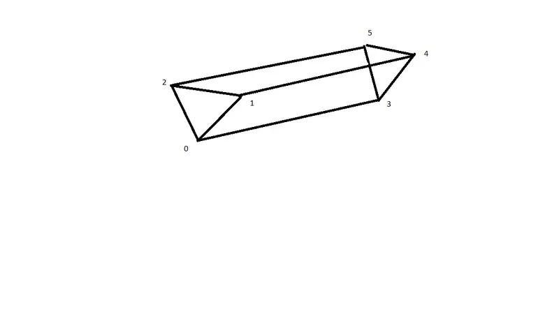
in the above figure, the line 2-1 and 4-5 are actually an arc
as we can see this will be our geometry and in this figure, we have specified the vertices that will be used to create the blockMeshDict. in this project, we will be creating the blockMeshDict txt file using Matlab
Matlab program for blockMeshDict:
clear all
close  all
clc
%this are some assumption made in dimension to perform simulation
re=2100;%reyolnds number for this given flow
D=0.019;%diameter of the pipe in meters
R=D/2;
l_h=0.05*re*D;%this is hydrodynamic length
l=1+l_h;%length of the pipe in meters assumed such that it is greater than l_h
theta=3;%wedge angle <5 degee

y=D*0.5*cosd(theta\2);
z=D*0.5*sind(theta\2);
%vertex of the point which represents asixymetric diagram of the pipe
vt0=[0,0,0];
vt1=[0,y,z];
vt2=[0,y,-z];
vt3=[l,0,0];
vt4=[l,y,z];
vt5=[l,y,-z];
f1= fopen('blockMeshDict','w');
fprintf(f1,'FoamFile');
fprintf(f1,'\n');
fprintf(f1,'{');
fprintf(f1,'\n');
fprintf(f1,'version     2.0;');
fprintf(f1,'\n');
fprintf(f1,'format      ascii;');
fprintf(f1,'\n');
fprintf(f1,'class       dictionary;');
fprintf(f1,'\n');
fprintf(f1,'object      blockMeshDict;');
fprintf(f1,'\n');
fprintf(f1,'} \n');
fprintf(f1,'convertToMeters 1; \n')
fprintf(f1,'\n');
fprintf(f1,'vertices');
fprintf(f1,'\n');
fprintf(f1,'( \n');
fprintf(f1,'(%f %f %f)\n',vt0(1),vt0(2),vt0(3)); %zeroth vertex
fprintf(f1,'(%f %f %f)\n',vt1(1),vt1(2),vt1(3));%1st vertex
fprintf(f1,'(%f %f %f)\n',vt2(1),vt2(2),vt2(3));%2nd vextex
fprintf(f1,'(%f %f %f)\n',vt3(1),vt3(2),vt3(3));%3rd vertex
fprintf(f1,'(%f %f %f)\n',vt4(1),vt4(2),vt4(3));%4th vertex
fprintf(f1,'(%f %f %f)\n',vt5(1),vt5(2),vt5(3));%5th vertex
fprintf(f1,'); \n');
fprintf(f1,'blocks\n');
fprintf(f1,'( \n');
fprintf(f1,'hex (0 2 1 0 3 5 4 3) (20 1 100)  simpleGrading (1 1 1) \n');
fprintf(f1,');\n');
fprintf(f1,'edges \n (\n');
fprintf(f1,'\t %s (0 %d 0)\n','arc 1 2 ',R);
fprintf(f1,'\t %s (%d %d 0)\n','arc 4 5 ',l,R);
fprintf(f1,');\n');
fprintf(f1,'boundary \n ( \n inlet \n { \n type patch;\n faces \n ( \n');
fprintf(f1,'(0 1 2 0)\n ); \n }\n');
fprintf(f1,'outlet \n { \n type patch;\n faces \n( \n (3 5 4 3) \n );\n }\n');
fprintf(f1,'top \n { \n type patch;\n faces \n( \n  (1 4 5 2) \n );\n }\n');
fprintf(f1,'wedgeFornt \n { \n type wedge;\n faces \n( \n (0 2 5 3) \n );\n }\n');
fprintf(f1,'wedgeBack \n { \n type wedge;\n faces \n( \n (0 1 4 3) \n );\n }\n');
fprintf(f1,'bottom \n { \n type empty;\n faces \n( \n (0 3 3 0) \n );\n }\n );\n */');
fprintf(f1,'mergePatchPairs \n( \n );\n');
fclose(f1);
blockMeshDict:
note: in this blockmeshdict, only executable lines are written In the Matlab program
FoamFile
{
version     2.0;
format      ascii;
class       dictionary;
object      blockMeshDict;
}
convertToMeters 1;

vertices
(
(0.000000 0.000000 0.000000)
(0.000000 0.009499 0.000111)
(0.000000 0.009499 -0.000111)
(2.995000 0.000000 0.000000)
(2.995000 0.009499 0.000111)
(2.995000 0.009499 -0.000111)
);
blocks
(
hex (0 2 1 0 3 5 4 3) (20 1 100)  simpleGrading (1 1 1)
);
edges
 (
	 arc 1 2  (0 9.500000e-03 0)
	 arc 4 5  (2.995000e+00 9.500000e-03 0)
);
boundary
 (
 inlet
 {
 type patch;
 faces
 (
(0 1 2 0)
 );
 }
outlet
 {
 type patch;
 faces
(
 (3 5 4 3)
 );
 }
top
 {
 type patch;
 faces
(
  (1 4 5 2)
 );
 }
wedgeFornt
 {
 type wedge;
 faces
(
 (0 2 5 3)
 );
 }
wedgeBack
 {
 type wedge;
 faces
(
 (0 1 4 3)
 );
 }
bottom
 {
 type empty;
 faces
(
 (0 3 3 0)
 );
 }
 );
 */mergePatchPairs
(
 );
Transport properties:
here the kinematic viscosity of the water at 30 degrees is been considered
/*--------------------------------*- C++ -*----------------------------------*\
  =========                 |
  \\      /  F ield         | OpenFOAM: The Open Source CFD Toolbox
   \\    /   O peration     | Website:  https://openfoam.org
    \\  /    A nd           | Version:  8
     \\/     M anipulation  |
\*---------------------------------------------------------------------------*/
FoamFile
{
    version     2.0;
    format      ascii;
    class       dictionary;
    location    "constant";
    object      transportProperties;
}
// * * * * * * * * * * * * * * * * * * * * * * * * * * * * * * * * * * * * * //

nu              [0 2 -1 0 0 0 0] 8.01e-07;


// ************************************************************************* //
Boundary conditions:
Initial velocity :
/*--------------------------------*- C++ -*----------------------------------*\
  =========                 |
  \\      /  F ield         | OpenFOAM: The Open Source CFD Toolbox
   \\    /   O peration     | Website:  https://openfoam.org
    \\  /    A nd           | Version:  8
     \\/     M anipulation  |
\*---------------------------------------------------------------------------*/
FoamFile
{
    version     2.0;
    format      ascii;
    class       volVectorField;
    object      U;
}
// * * * * * * * * * * * * * * * * * * * * * * * * * * * * * * * * * * * * * //

dimensions      [0 1 -1 0 0 0 0];

internalField   uniform (0 0 0);

boundaryField
{
    inlet
    {
        type            fixedValue;
        value           uniform (0.16821 0 0);
    }

    outlet
    {
        type            zeroGradient;

    }

    wedgeFornt
    {
        type            wedge;
    }

    wedgeBack
    {

    type              wedge;

    }

    top
    {

    type               noSlip;


     }

     bottom
     {

     type         empty;
     }


}

// ************************************************************************* //
initial pressure condition:
/*--------------------------------*- C++ -*----------------------------------*\
  =========                 |
  \\      /  F ield         | OpenFOAM: The Open Source CFD Toolbox
   \\    /   O peration     | Website:  https://openfoam.org
    \\  /    A nd           | Version:  8
     \\/     M anipulation  |
\*---------------------------------------------------------------------------*/
FoamFile
{
    version     2.0;
    format      ascii;
    class       volScalarField;
    object      p;
}
// * * * * * * * * * * * * * * * * * * * * * * * * * * * * * * * * * * * * * //

dimensions      [0 2 -2 0 0 0 0];

internalField   uniform 0;

boundaryField
{
    inlet
    {
        type            zeroGradient;

    }

    outlet
    {
        type            fixedValue;
        value           uniform  0 ;

    }

    wedgeFornt
    {
        type            wedge;
    }

    wedgeBack
    {

    type              wedge;

    }

    top
    {

    type                zeroGradient;

     }

     bottom
     {

     type              empty;
     }
}

// ************************************************************************* //
time step and total simulation time :
/*--------------------------------*- C++ -*----------------------------------*\
  =========                 |
  \\      /  F ield         | OpenFOAM: The Open Source CFD Toolbox
   \\    /   O peration     | Website:  https://openfoam.org
    \\  /    A nd           | Version:  8
     \\/     M anipulation  |
\*---------------------------------------------------------------------------*/
FoamFile
{
    version     2.0;
    format      ascii;
    class       dictionary;
    location    "system";
    object      controlDict;
}
// * * * * * * * * * * * * * * * * * * * * * * * * * * * * * * * * * * * * * //

application     icoFoam;

startFrom       startTime;

startTime       0;

stopAt          endTime;

endTime         10;

deltaT          1e-03;

writeControl    timeStep;

writeInterval   200;

purgeWrite      0;

writeFormat     ascii;

writePrecision  6;

writeCompression off;

timeFormat      general;

timePrecision   6;

runTimeModifiable true;


// ************************************************************************* //
Mesh:
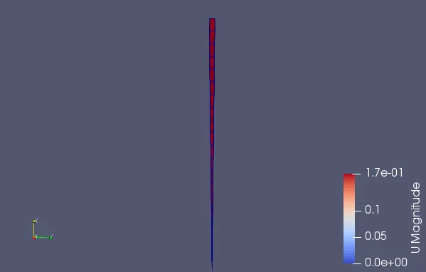
inlet :
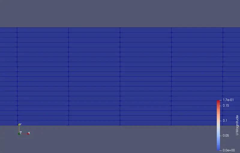
along the length of the pipe :
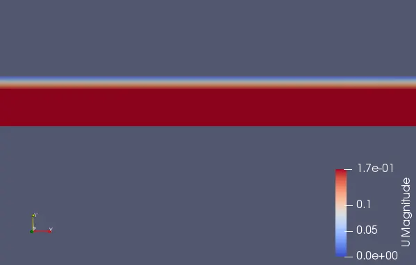
after simulation:
Discussion of graphs:
1. validating hydrodynamic length with the numerical result
as we know the hydrodynamic length for laminar flow can be calculated analytically using the formula `(L_h)/D=0.05*Re`
in our problem, the diameter of the pipe is 0.019m and the Reynolds number is 2100 then L_h=1.995 `~=2`
note: L_h is the dimensionless length
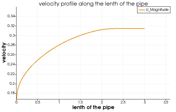
as we can see the above graph represents velocity along the length of the pipe and by looking at the graph we can say that the maximum velocity is changing from the inlet of the pipe. after 2 meters the velocity is constant which indicates that up to 2 m the flow region is the hydrodynamic entrance region and after 2 m the flow is a fully developed flow that after that the wall shear stress is constant so the maximum velocity will be constant after that region which can be seen in this graph
2. validating the fully developed velocity profile :
as we know for fully developed flow the velocity profile along the pipe will not change that is `(delu(x,r))/(delx)=0` so u=u(r) means the change in velocity will only be in the radial direction.
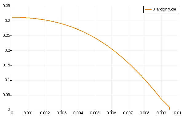
this is the velocity profile at the hydrodynamic length as we can see it parabolic since we are a simulation for a section of pipe we will get this half parabola.u(r)=`2*v_(avg)` this is for fully developed flow so let's check it for r=0 m means at the center of the pipe.
note: the general velocity profile formula for pipe is u(r)=`2*v_(avg)*(1-(r^2)/R^2)` where R is the radius of the pipe and r is the distance from the center of the pipe along radial axis fr which we need to know the velocity profile
we know that the average velocity of the flow is 0.1681 m/s. u(0)=2*0.1681=0.3362 m/s this is the analytical result and by observing the plot our analytical result and our result obtained by simulation are approximately equal
3. Validate maximum velocity and pressure drop for fully developed flow :
as we saw in the second validation the maximum velocity occurs in the centerline which we call u_max and it is given by the formula u_max=2v_avg which has been validated in the above section.
for pressure drop, the analytical result is obtained from the Hagen-posicllues equation `v_(avg)*A_c=(/_\p*pi*D^4)/(128muL)` and by rearranging we get `(v_(avg)*A_c*128*mu*L)/(pi*D^4)=/_\p` and from this, we can say that the average velocity, area of cross-section, the diameter of the pipe, the dynamic viscosity of the fluid are constant at the fully developed region so the pressure drop is only depending on the length of the pipe this means pressure drop is directly proportional to the length of the pipe we can also say that as we move along the length of the pipe from the inlet of the fluid the pressure drop increases and thus required extra pumping power. and graphically it should be linear.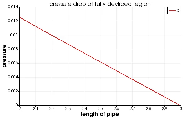
from this plot, we can say that our analytical meaning of the pressure drop and graphical meaning is the same.
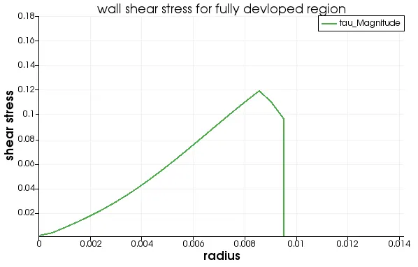
4. Post-process Shear stress and validate wall shear stress for fully developed flow:
the shear stress for this flow is `tau=mu*(du)/(dy)` and the wall shear stress need to be maximum at the wall of the pipe and it should be less as we move towards the radial direction from the wall (top face)
post-processing of wall shear stress :
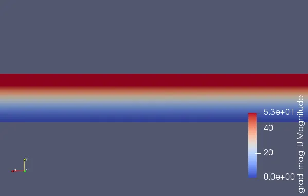
as we can see in the above picture the shear stress at the wall is high as we move down the shear stress is decreasing and at the center of the pipe (r=0), the shear stress is almost 0.
the plot of the wall shear stress along the radial direction in the fully developed region