Solving the steady and unsteady 2D heat conduction problem using MATLAB.
Mid-Term Project Report
- Aim: To solve the steady and unsteady 2D heat conduction Equation and then plotting contours to study the results.
- Theoretical Introduction:
Thermal conduction is the transfer of internal energy by microscopic collisions of particles and movement of electrons within a body. The colliding particles, which include molecules, atoms and electrons, transfer disorganized microscopic kinetic and potential energy, jointly known as internal energy. Conduction takes place in all phases: solid, liquid, and gas.
Heat spontaneously flows from a hotter to a colder body. For example, heat is conducted from the hotplate of an electric stove to the bottom of a saucepan in contact with it. In the absence of an opposing external driving energy source, within a body or between bodies, temperature differences decay over time, and thermal equilibrium is approached, temperature becoming more uniform.
In conduction, the heat flow is within and through the body itself. In contrast, in heat transfer by thermal radiation, the transfer is often between bodies, which may be separated spatially. Also possible is the transfer of heat by a combination of conduction and thermal radiation. In convection, the internal energy is carried between bodies by a moving material carrier. In solids, conduction is mediated by the combination of vibrations and collisions of molecules, of propagation and collisions of phonons, and of diffusion and collisions of free electrons. In gases and liquids, conduction is due to the collisions and diffusion of molecules during their random motion. Photons in this context do not collide with one another, and so heat transport by electromagnetic radiation is conceptually distinct from heat conduction by microscopic diffusion and collisions of material particles and phonons. But the distinction is often not easily observed unless the material is semi-transparent.
For Steady State conduction:
Equation for 2Dimensional Steady State Conduction: `(del^2T)/(delx^2)+ (del^2T)/(dely^2) = 0`
Steady-state conduction is the form of conduction that happens when the temperature difference(s) driving the conduction are constant, so that (after an equilibration time), the spatial distribution of temperatures (temperature field) in the conducting object does not change any further. Thus, all partial derivatives of temperature concerning space may either be zero or have nonzero values, but all derivatives of temperature at any point concerning time are uniformly zero. In steady-state conduction, the amount of heat entering any region of an object is equal to the amount of heat coming out (if this were not so, the temperature would be rising or falling, as thermal energy was tapped or trapped in a region).
For Unsteady State or Transient state Conduction:
During any period in which temperatures changes in time at any place within an object, the mode of thermal energy flow is termed transient conduction. Another term is "non-steady-state" conduction, referring to time-dependence of temperature fields in an object. Non-steady-state situations appear after an imposed change in temperature at a boundary of an object. They may also occur with temperature changes inside an object, as a result of a new source or sink of heat suddenly introduced within an object, causing temperatures near the source or sink to change in time.
When a new perturbation of temperature of this type happens, temperatures within the system change in time toward a new equilibrium with the new conditions, provided that these do not change. After equilibrium, heat flow into the system once again equals the heat flow out, and temperatures at each point inside the system no longer change. Once this happens, transient conduction is ended, although steady-state conduction may continue if heat flow continues.
Equation for 2Dimensional Unsteady State Conduction: `(delT)/(delt) = alpha((delT^2)/(delx^2)+ (delT^2)/(dely^2))` - Code/Logic:
1. We firstly need to clear and close all the previously entered codes and the present values of the already used variables, hence we use the following commands:
clear all
close all
clc
2. We then start the code by giving all the necessary inputs that are required to solve the equation. We must also add some comments so that we understand the code even better for further reference. Adding comments makes the code easy to read for any other user who is going to read the code as well.
Some of these inputs are as follows:
nx=10 - Number of Grid points along the x-direction
ny=10 - Number of Grid points along the y-direction
T_T = 600 - Temperature at the top of the domain.
T_B = 900 - Temperature at the Bottom of the domain.
T_L = 400 - Temperature at the Left Hand side of the domain.
T_R = 800 - Temperature at the Right Hand side of the domain.
tol = 1e-4 - Set Tolerance.
L = 1 - Length of the domain.
There are other Inputs along these that will help us solve the equation. We must mention the Iteration counter for every method. Like for example, for the Jacobian Method, we set the Iterative counter in a variable as: Jacobian_Iter. Just like this, we can set the Iteration counter for every loop.
3. After giving the inputs, we then go onto calculate the basic properties such as the delx and dely for the domain. Now, we must give in the formula for these calculations as well. The formulae are given below:
delx= L/nx - Scattered points in the X-Direction.
dely=L/ny - Scattered points in the Y-Direction.`k=2*((delx)^2+ (dely)^2)/((delx)^2*(dely)^2)` Here, k is a constant.
Another important step is to create the Temperature Matrix. To do this, we use the ones command and then multiply the ones with an initial estimate guess of 300K.
The Interesting thing to note here is that as the initial guess temperature gets closer to the Final Steady state temperature, the Number of iterations will reduce. Meaning, if the guess Temperature is closer to the actual value of the Steady State Temperature, the number of iterations to solve the equation for this value will be much lesser.
4. Then, in the next step, we will set a for loop that will run between 1 and the length of the Iterative_solver. We have set the variable as having an array as [1,2,3]. Here, as the for loop will run for e=1, e=2 and then finally e=3, our Iterative Solver method will change from Jacobian, Gauss-Siedel to Successive Solver method respectively.
All the Iterative Solvers have been put in this loop and then the results are plot for them as well. The Fundamental Difference between these methods is that In the Jacobian Method, we use all the values from the Previous iteration, whereas in the Gauss-Siedel Method, we update the values and use these values from the previous location within the same iteration. In the Successive Relaxation method, we simply enhance the performance of these two iterative solvers by giving a Relaxation factor to the equation.
The codes are mentioned in the main code box below.
Main Code(Steady State Equation)
%Solving for the Steady 2D Heat Conduction Equation clear all close all clc %Inputs nx=10; %Number of Grid points along the x-direction ny=10; %Number of Grid points along the y-direction T_T = 600; %Temperature at the top of the domain. T_B = 900; %Temperature at the Bottom of the domain. T_L = 400; %Temperature at the Left Hand side of the domain. T_R = 800; %Temperature at the Right Hand side of the domain. tol = 1e-4; %Set Tolerance. L = 1; %Length of the domain. x = linspace(0,L,nx); %Grid points evenly spaced along the Domain in X-Axis. y = linspace(0,L,ny); %Grid points evenly space along the Domain in Y-Axis. y= flip(y); %Flipping the y-domain for plotting. Error = 9e9; %Error Defined to start the while loop. Iterative_solver = [1,2,3]; %Value to solve for different methods. q = 1.2; %Relaxation Factor for SOR Method. Jacobian_Iter = 1; %Setting the Iteration counter GS_Iter = 1; %Setting the Iteration counter SOR_Iter = 1; %Setting the Iteration counter %Solving for Steady State 2-Dimensional Heat conduction equation. %Eqn=d^2T/dx^2 + d^2T/dy^2 delx= L/nx; %Scattered points in the X-Direction. dely=L/ny; %Scattered points in the Y-Direction. k= 2*((delx)^2+ (dely)^2)/((delx)^2*(dely)^2); %constant T=300*(ones(nx,ny)); %Creating the Temperature Matrix T(:,1)= T_L; %Assigning Boundary Conditions. T(:,end) = T_R; %Assigning Boundary Conditions. T(1,:)= T_T; %Assigning Boundary Conditions. T(end,:) = T_B; %Assigning Boundary Conditions. T_initial = T; %Creating Copies of the original Temperature Matrix T_old = T; %Creating Copies of the original Temperature Matrix %Convergence loop %Method1= Jacobian Technique for e = 1:length(Iterative_solver) if Iterative_solver(e) == 1 tic; while Error > tol for i = 2:nx-1 for j = 2:ny-1 T(i,j) = (1/k)*((T_old(i-1,j) + T_old(i+1,j))/(delx^2) + (T_old(i,j+1)+T_old(i,j-1))/(dely^2)); end end Error = max(max(abs(T_old - T))); T_old = T; Jacobian_Iter = Jacobian_Iter + 1; time = toc; figure(1) [C,h] = contourf(x,y,T); clabel(C) colorbar title(['Jacobian Method'],['Simulation Time= ', num2str(time)]) end end %Method2= Gauss-Seidel Method if Iterative_solver(e) == 2 tic; Error = 9e9; T_old= T_initial; while Error > tol for i = 2:nx-1 for j = 2:ny-1 T(i,j) = (1/k)*((T(i-1,j) + T_old(i+1,j))/(delx^2) + (T_old(i,j+1)+T(i,j-1))/(dely^2)); end end Error = max(max(abs(T_old - T))); T_old = T; GS_Iter = GS_Iter + 1; time = toc; figure(2) [C,h] = contourf(x,y,T); clabel(C) colorbar title(['Gauss Seidel Method'],['Simulation Time= ', num2str(time)]) end end %Method3= Successive-Over Relaxation Method. if Iterative_solver(e) == 3 tic; Error = 9e9; T_old = T_initial; while Error > tol for i = 2:nx-1 for j = 2:ny-1 T(i,j) = (1-q)*(T_old(i,j)) + (q)*((1/k)*((T(i-1,j) + T_old(i+1,j))/(delx^2) + (T_old(i,j+1)+T(i,j-1))/(dely^2))); end end Error = max(max(abs(T_old - T))); T_old = T; SOR_Iter = SOR_Iter + 1; time= toc; figure(3) [C,h] = contourf(x,y,T); clabel(C) colorbar title(['Successive Over Relaxation Method'],['Simulation Time= ', num2str(time)]) end end end %END
Similarly for the Unsteady/Transient Method:
%Solving for the Unsteady 2D Heat Conduction Equation clear all close all clc %Inputs nx = 10; %Number of Grid points along the x-direction ny = 10; %Number of Grid points along the y-direction T_T = 600; %Temperature at the top of the domain. T_B = 900; %Temperature at the Bottom of the domain. T_L = 400; %Temperature at the Left Hand side of the domain. T_R = 800; %Temperature at the Right Hand side of the domain. tol = 1e-4; %Set Tolerance. L = 1; %Length of the domain. delx = L/nx; %Scattered points in the X-Direction. dely = L/ny; %Scattered points in the Y-Direction. x = linspace(0,L,nx); %Grid points evenly spaced along the Domain in X-Axis. y = linspace(0,L,ny); %Grid points evenly space along the Domain in Y-Axis. y=flip(y); %Flipping the y-domain. Error = 9e9; %Error Defined to start the while loop. T=300*(ones(nx,ny)); %Creating the Temperature Matrix T(:,1)= T_L; %Assigning Boundary Conditions. T(:,end) = T_R; %Assigning Boundary Conditions. T(1,:)= T_T; %Assigning Boundary Conditions. T(end,:) = T_B; %Assigning Boundary Conditions. T_initial = T; %Creating Copies of the original Temperature Matrix T_old = T; %Creating Copies of the original Temperature Matrix e = 1.4; %Diffusion Coefficient. delt = 0.001; %Time-step set k1 = e*(delt)/(delx^2); %CFL number along the X-direction. k2 = e*(delt)/(dely^2); %CFL number along the Y-direction. %Solving for the Unsteady State Solution %Eqn = delT/delt = e*(del^2(T)/delx^2 + del^2(T)/dely^)2) %For the Explicit Method. %Convergence Loop. %Time Loop for nt=1:1000 for i = 2:nx-1 for j = 2:ny-1 T(i,j) = T_old(i,j) + (k1)*(T_old(i-1,j)- (2*T_old(i,j))+ T_old(i+1,j)) + (k2)*(T_old(i,j+1)-(2*T_old(i,j))+T_old(i,j-1)); end end T_old = T; %Updating the value after every Iteration. end figure(1) [C,h] = contourf(x,y,T); clabel(C) colorbar title('Explicit Method') %For Implicit Method T_prev = T_old; for nt= 1:1000 Error = 9e9; T_old = T_initial; while Error>tol term1 = 1/(1+ 2*(k1)+ 2*(k2)); term2 = k1*term1; term3= k2*term1; for i = 2 : nx-1 for j = 2 : ny-1 T(i,j) = term1 * T_prev(i,j) + term2 * (T_old(i-1,j)+ T_old(i+1,j)) + term3 * (T_old(i,j+1)+T_old(i,j-1)); end end Error= max(max(abs(T_old-T))); T_old = T; %Updating the value after every Iteration. end T_prev = T; %Updating the value after every Time-Step. end figure(2) [C,h] = contourf(x,y,T); clabel(C) colorbar title('Implicit Method') %END - Results:
We get the following plots:
a. For Steady State Equation
a.1) Jacobian Method: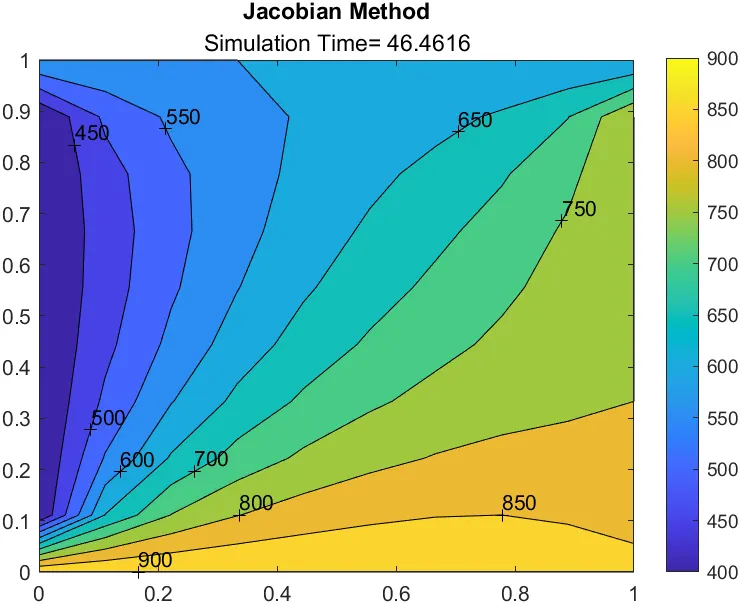
a.2)Gauss-seidel Method: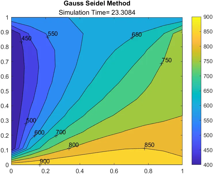
a.3)Successive Over Relaxation Method: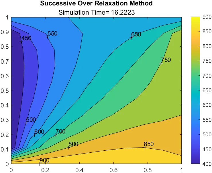
As we can see from the plots that the Simulation time is decreasing as we move from the jacobian method to the Gauss-Seidel Method and finally to the Successive Over Relaxation Method. The Simulation time for Jacobian Method is approximately 46 seconds and in the case of Gauss-Seidel Method, the simulation time decreases to almost half of the Jacobian Method to at around 23 seconds. In the case of Successive Over Relaxation method, the Simulation time is around 16 seconds.
Hence out of all the three Methods, the Successive Over-Relaxation method produces the fastest results. We basically get the same final output, but we achieve this by using different methods.
b.)For UnSteady State Equation
We can solve this equation by two methods specifically, they are:
b.1)Explicit Method: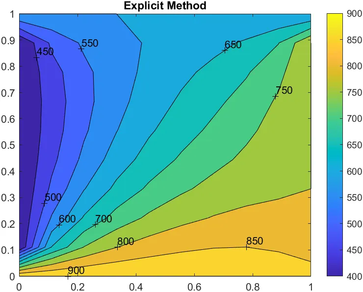
b.2)Implicit Method: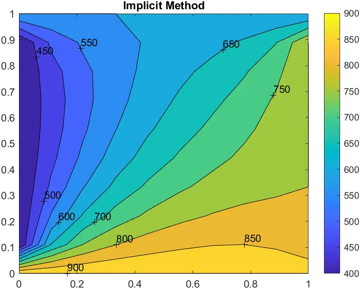
- Conclusion: In conclusion, I would like to state that this project helped me understand how the Heat conduction equation can be solved in the case of both, the steady and the unsteady conditions. In this project, we understand that as the initial guess temperature gets closer to the Final Steady state temperature, the Number of iterations will decrease for the simulation, but the Simulation time will remain the same.