Week 4- Rolling operation

Objective

We have to simulate the rolling operation on a workpiece made of copper. The model will be provided to you. Increase the length of the

workpiece by 60mm and decrease its size on both sides by 8mm. Run the simulation for 14 steps and you can give small but random values(

similar to the ones mentioned in the video) for the displacement. Ensure that the edge of the workpiece is displaced by 90mm.

Geometry:

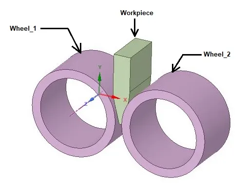
In geometry, there are two Roll Wheels and one Workpiece as shown in below image.

_______________________________________________________________________________________________________

Material Specifications:

Copper Alloy NL

Density: 8300 Kg/m³

Young’s Modulus: 1.1 E+05 MPa

Poisson’s Ratio: 0.34

Yield Strength: 280 MPa

Tangent Modulus: 1150 Mpa

_______________________________________________________________________________________________________

Mesh

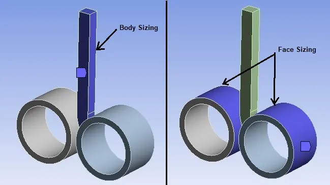
Details:

• Global Element Size: Default
• Body Sizing : Workpiece

Element Size = 1.5 mm

• Face Sizing : Wheel_1 & Wheel_2

Element Size = 2.5 mm

• No. of Nodes: 35616
• No. of Elements: 6763

________________________________________________________________________________________________________________________

Procedure:

• Import model in Static Structural named as “Skill_Lync_Copper_Rolling.stp” in Geometry section.
• Change in the geometry as follows:
• Increase length of Copper Workpiece by 60 mm.
• Decrease width of Copper Workpiece by 8 mm on both sides.

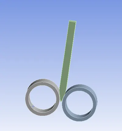
• We can see that final thickness of Copper rode has been 9 mm.
• Then go to Mechanical model section.
• Rename Roll Wheels and Copper rod as Wheel_1, Wheel_2 and Workpiece as shown above in geometry.

Connections:

• Delete automatically created contacts and create new contacts as given below:

Contact_1:

Contact Body = WORK_PIECE

Target Body = WHEEL_1

Contact_2:

Contact Body = WORK_PIECE

Target Body = WHEEL_2

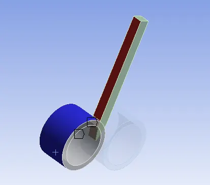
FIG:CONTACT 1

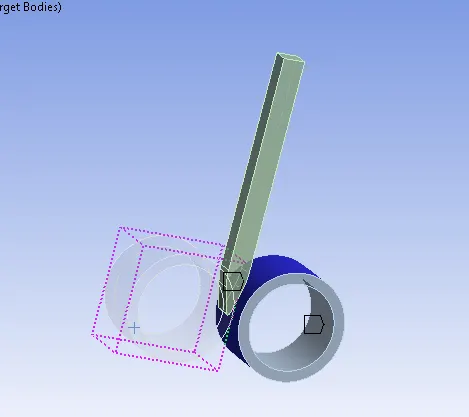
FIG:CONTACT 2

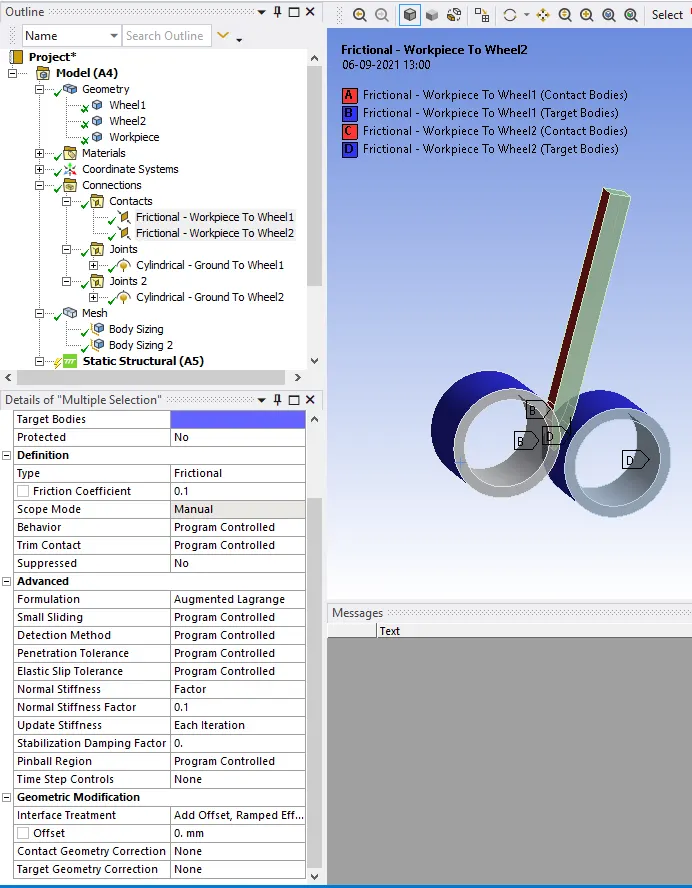
Settings for both Contacts:

• Type: Frictional
• Friction Coefficient: 0.1
• Formulation: Augmented Lagrange
• Normal Stiffness : By factor
  • Normal Stiffness Factor: 0.1
• Update Stiffness: Each Iteration
• Interface Treatment: Add Offset, Ramped Effects

Joints:

Joint_1

Connection Type: Body-Ground

Type: Cylindrical

Body: Wheel_1

Joint_2

Connection Type: Body-Ground

Type: Cylindrical

Body: Wheel_2

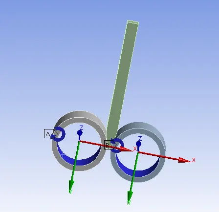
• Change the direction of Z-axis as per above image.

Boundary Conditions:

• After meshing as described above, create Boundary Conditions as given below:

Analysis Settings:

• Number of Steps: 14
• Auto Time Stepping: Program Controlled
• Solver Type: Program Controlled
• Large Deflection: ON
• Nonlinear Controls:
  • Stabilization: Constant
  • Method: Energy
  • Energy Dissipation Ratio: 0.1
• Other Boundary conditions for joints are as given below:
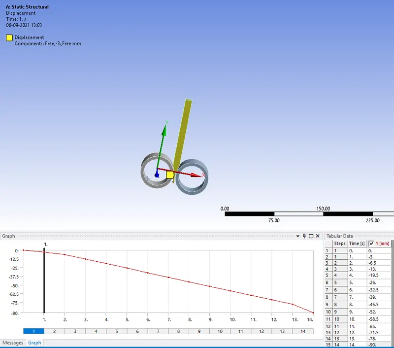
• Now we want to move the workpiece between two wheels up to 90 mm, so we have to give it a displacement.

Displacement:

Direction: -Y (Negative)

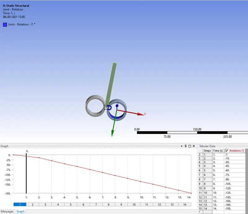
Joint Load_1:

Joint: Revolute – Ground to Wheel_1

Type: Rotation

Magnitude: Tabular Data

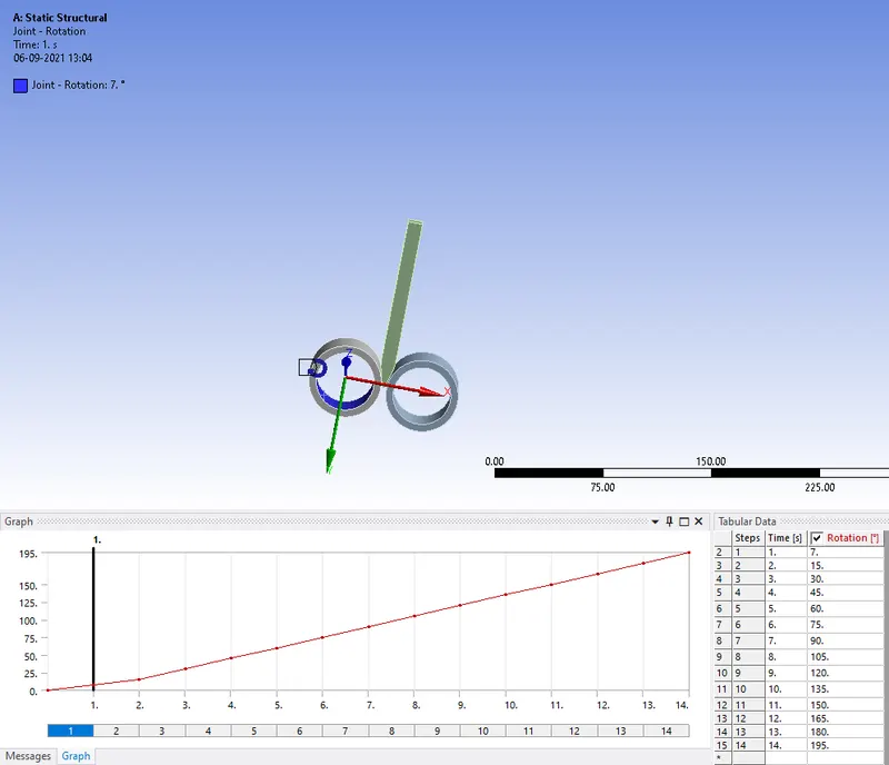
Joint Load_2:

Joint: Revolute – Ground to Wheel_2

Type: Rotation

Magnitude: Tabular Data

Solution:

• After giving proper boundary conditions, create desired solutions for output results.
• Create Solutions for :
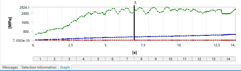
  • Equivalent Stress For Whole Setup
  • Equivalent Plastic Strain for the Workpiece
  • Directional Deformation in Z-axis for the Workpiece
  • Directional Deformation in Y-axis for the Workpiece

________________________________________________________________________________________________________________________

Results:

Now we will see the results for requested solutions.

Stress Contours (Whole Setup):

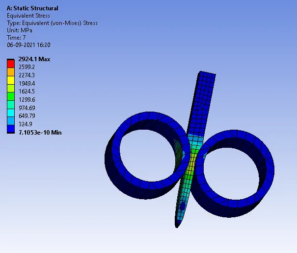
Stress Plot (Whole Setup):

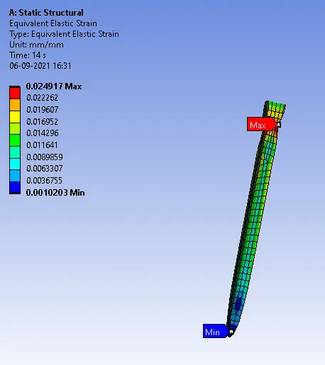
Plastic Strain (Workpiece):

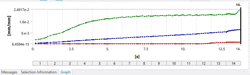
Plastic Strain Plot (Workpiece):

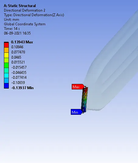
Directional Deformation in Z-Axis (Workpiece):

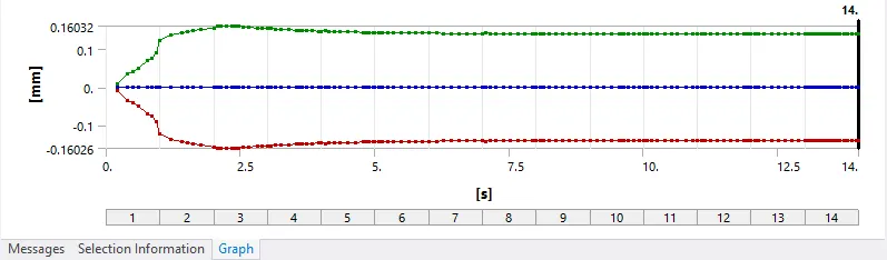
Directional Deformation) in Z-Axis Plot (Workpiece):

Proof for Displacement of Workpiece up to 90mm:

• Now we want to verify that workpiece has moved or displaced up to 90 mm in Y – Axis direction.
• As we know, we have given Displacement to Workpiece up to 90 mm.
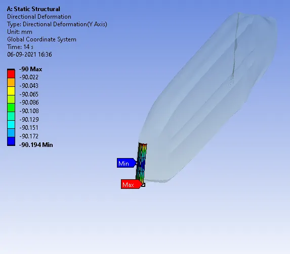
• To verify it, we will see the Direction Deformation of the Workpiece and see that the Tip of the Workpiece has displaced up to 90mm or not.

Directional Deformation in Y-Axis (Workpiece):

Directional Deformation) in Y-Axis Plot (Workpiece):

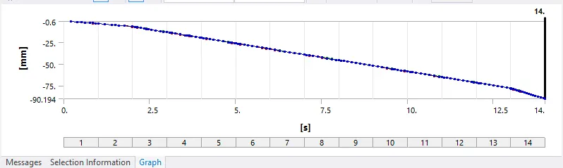
• Here in above contours image, we can see that Maximum displacement of the tip of the workpiece is 90 mm Maximum.
• Also maximum deformation can be observed from the above plot.
• This is the proof that Workpiece has displaced up to 90mm.

_ _ _ _ _ _ _ _ _ _ _ _ _ _ _ _ _ _ _ _ _ _ _ _ _ _ _ _ _ _ _ _ _ _ _ _ _ _ _ _ _ _ _ _ _ _ _ _ _ _ _ _ _ _ _ _ _ _ _ _ _ _ _ _ _ _ _ _ _ _ _ _ _ _ _ _ _ _ _ _ _ _ _ _ _ _

Draught:

The difference between the thickness of initial and rolled metal piece is called Draught. Thus if t₀ initial thickness and t_f is final thickness, then the draught d is given by

d = t₀ - t_f

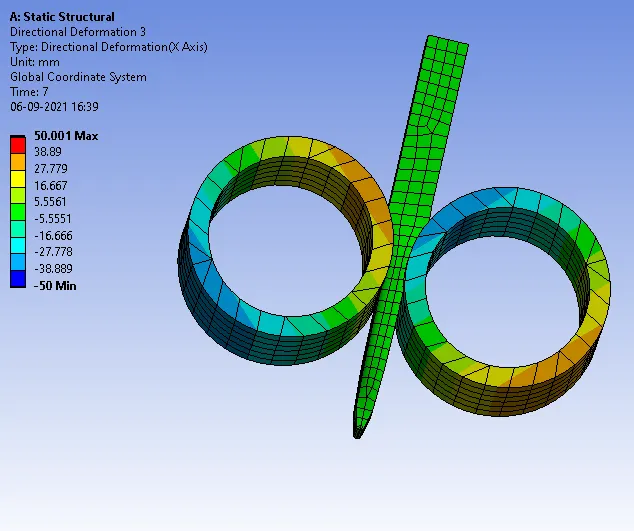
• Here we can check thickness change by seeing the result of directional deformation in X-Axis.

So_, in this case,

T₀ = initial thickness / length = 10 mm

T_f = final thickness / length = 4 mm (decreased 3 mm each side)

d = 10 – 4

d = 6 mm

For Maximum Draught,

d _max = f² * R

R= Radius of Roller

F = Static friction coefficient

R = 25 mm

F = 0.2

So,

d _{max =} (0.2)² * 25 = 1 mm.

• So we can get Minimum thickness or Maximum Draught from rolling Process = 1 mm.

________________________________________________________________________________________________________________________

Conclusion:

This study of the rolling process drew every minute aspect. In terms of manufacturing engineering, every engineer should consider the rolling

process as a core metal forming process. This process is mainly used when a cross-sectional area of a material required to be changed by an

engineer.