Week 4: Project - Transient simulation of flow over a throttle body

FLOW OVER A THROTTLE BODY

AIM: To simulate the flow over an elbow of a throttle valve and post process the results in paraview. The simulation is done for two conditions i.e. steady- state and transient flow conditions.

THEORY: A throttle is derived from the word “throat” which means to regulate the flow of a fluid over a body. Similarly a throttle body consists of a butterfly valve that is a flow control valve that consists of a disc that can rotate to control the pressure and flow of a liquid. Butterfly valves are of different types and its application depends on the pipeline diameter. It has wide application in automobiles and it is used to improve the fuel- efficiency and curb emissions. When the engine is at relatively high RPM, there is relatively less time for the fuel to burn completely due to which a portion of the fuel goes unburnt thereby decreasing the fuel efficiency of the car. A throttle valve thereby detects the amount of fuel that is required for the engine to keep running directly based on the throttle provided on the pedal by the driver. In modern vehicles the throttle body itself is regulated by an ECU- engine control unit that decides the amount of fuel or air or the air/fuel ratio that is be taken in. Hence our main aim is to study and investigate the characteristics of the flow under a steady state and transient conditions

Transient flow: A flow where we the flow taking place is unsteady due to real life turbulences. If a variable defining the state of the system does not change with respect to time then it is called steady state flow

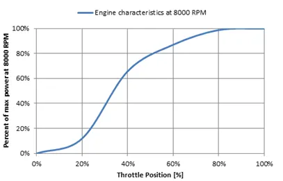
Figure 1: Flow over a throttle body

PROCEDURE:

• Import the STL file that was provided or sketch the geometry of the channel.

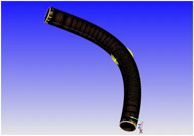
Figure 2: Geometry with translated normal

• Convert the units of the imported geometry to metres by using the scale option.
• Now translate the normal to the direction of the fluid flow.
• While setting up the case we select O2 and N2 as the fluid flowing through the geometry with their natural molar concentrations as 0.23 and 0.77 respectively.
• Setup the values for the steady state simulation. We consider the flow to be a taking place under 2 different condition i.e. steady-state and transient flow. A transient flow is carried out since in real time testing the throttle body is subjected to fluctuations owing to bad road conditions. Enter the number of cycles. I have assumed 20000 cycles with a sample size of 800.The inlet pressure is 1.5 bar and outlet pressure is 1 bar. This difference of 0.5 bar will drive the flow.
• Flag and assign the boundaries to the geometry.

• Enter the value for the base-grid for the simulation i.e. 4e-3.

• Under the case setup tree select fixed embedding and enter the scale to a value of 3. This is done to refine the mesh closer to the region of the throttle valve to improve the accuracy of the parameters that we will view after the simulation.

• Processing and post converting the input files using cygwin.

• Post processing using paraview. Obtain the velocity, pressure and glyph plots using paraview tools.

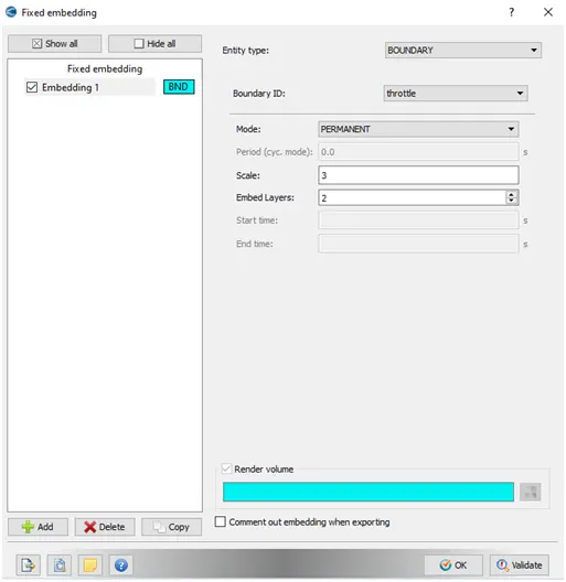
Figure 3: Fixed embedding window

PROCEDURE (TRANSIENT FLOW): The case-setup procedure for a transient flow simulation is similar to the steady state simulation. However we do make a few changes in the case setup procedure as listed below.

• Under run parameters we select the solver type as transient flow simulation.
• While assigning regions to the boundary we make sure to change the motion of the throttle to rotating and assign the rotation center and the axis of rotation. This is done by selecting 3 different points from the cylinder of the throttle valve by hiding all the other boundary conditions. Note that the rotation about the z axis is zero since the throttle rotates only in X-Y direction.

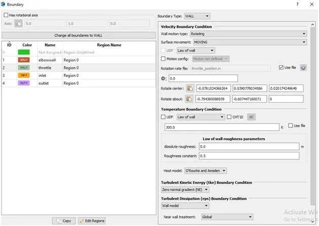
Figure 4: Throttle boundary condition for transient flow simulation

• Under the throttle boundary enter the throttle rotating rate. The assumed values are given below.

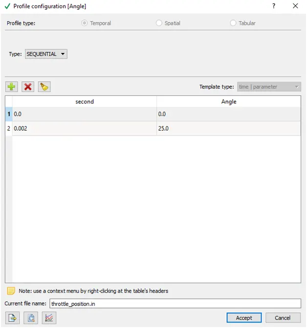
Figure 5: Throttle rotation rate

• Enter the writing time interval of output files as 0.001 seconds and the other parameters are set to the default values.

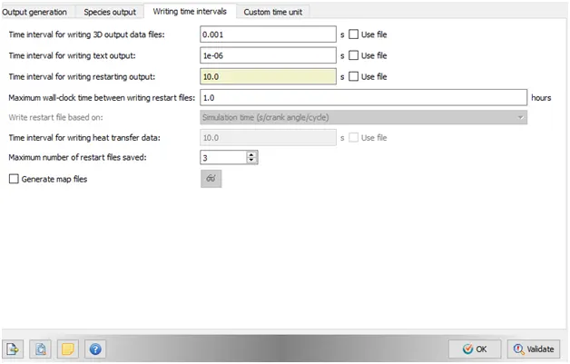
Figure 6: Time interval for writing 3D output files

• After following the above steps we export the input files to a folder and run the simulation in cygwin.

OBSERVATION: The velocity contour and the pressure contour has been obtained for steady state simulation and transient simulation.

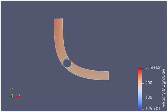
Figure 7: Velocity contour for a steady state case

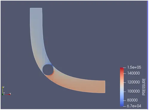
Figure 8: Pressure contour for a steady state simulation

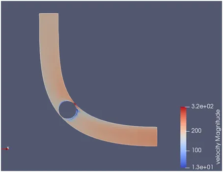
Figure 9: Velocity contour transient flow

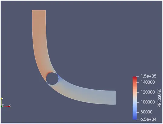
Figure 10: Pressure contour- transient case

PLOTS:

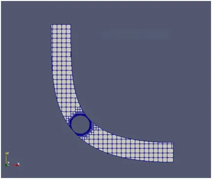
Figure 11: Mesh geometry with fixed embedding

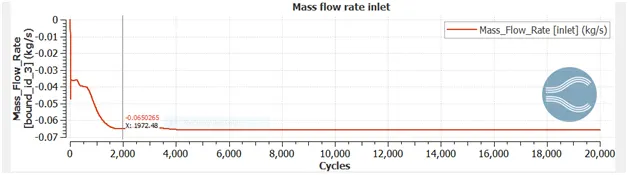
Figure 12: Mass flow rate inlet-steady state

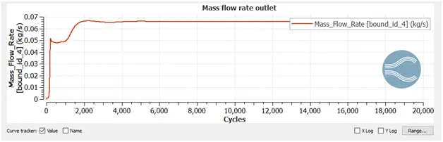
Figure 13: mass flow rate outlet-steady state

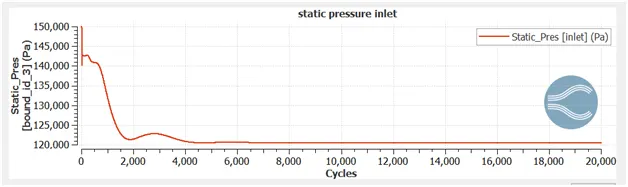
Figure 14: Static pressure inlet-steady state

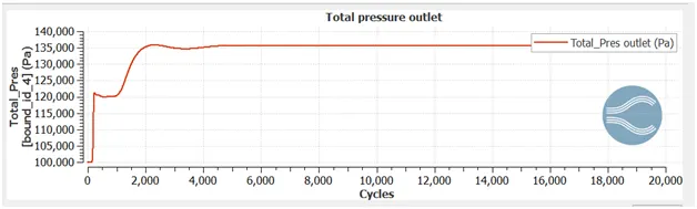
Figure 15: Total pressure outlet-steady state

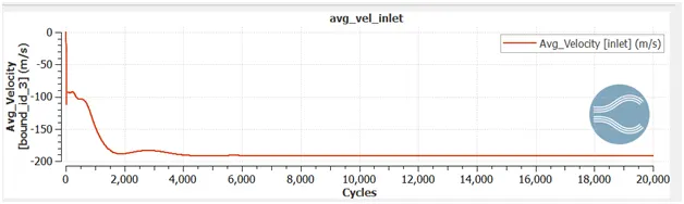
Figure 16:Avg velocity inlet-steady state

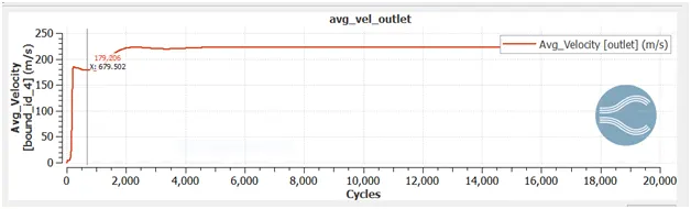
Figure 17: Avg velocity outlet-steady state

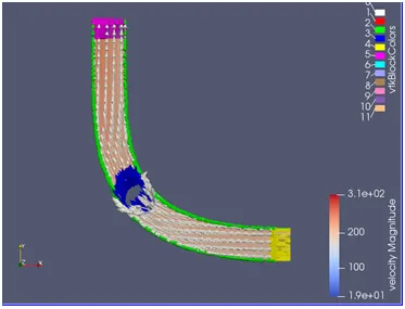
Figure 18: Velocity vectors for throttle flow

PLOTS (for transient case): The velocity, mass flow rate and the pressure plots have been shown below.

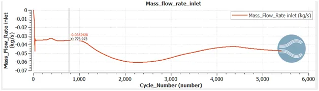
Figure 19: Mass flow rate inlet

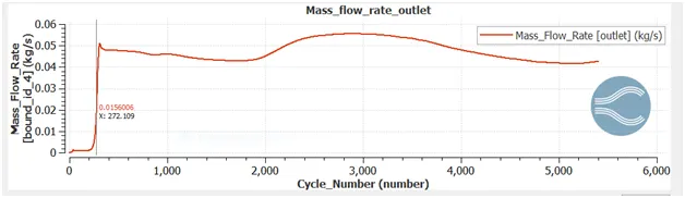
Figure 20: Mass flow rate outlet

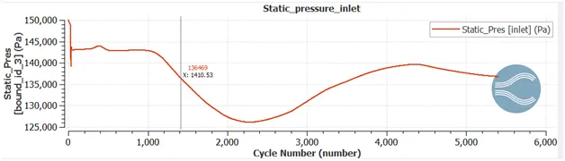
Figure 21: Static pressure inlet

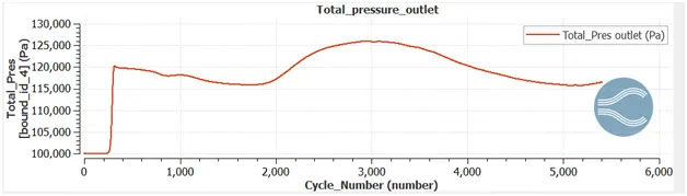
Figure 22: Total pressure outlet

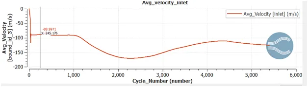
Figure 23: Avg velocity inlet

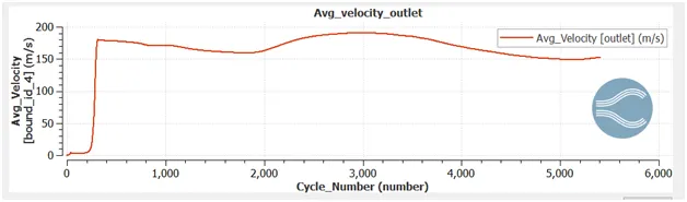
Figure 24: Average velocity outlet

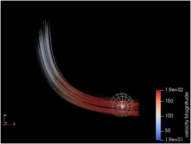
Figure 25: Glyph plot using stream tracer

CONCLUSION:

STEADY STATE CASE: From the plots that we can see from the steady state simulation cases we can see that the curves generally are smooth and lesser prone to anomalies. This is due to the increasing of the number of cells from the fixed embedding window by adjusting its scale. The number of cells is viewed using the Cartesian cell technique from converge studio. The velocity increases throughout the length of the elbow and as the flow gradually approaches the throttle plate the velocity decreases and so the pressure drastically increases because of sudden decrease in the area across the throttle valve. Later on the pressure, velocity and the mass flow restore their initial flow parameters as they gradually increasing after striking the throttle plate and reaching towards the outlet.

CONCLUSION (Transient case): In the transient simulation we have assumed that the throttle valve rotates by 25 degrees within 0.02 seconds. Initially when the valve was in open position there was not much of a difference between the entry and the exit of the elbow pipe. Now,as the valve rotates the throttle valve and the fluid flowing through it experiences high pressure. This is due to the fact that the total kinetic energy gets converted into the total pressure energy. The same cases happen with velocity and the mass flow rate. The velocity drastically reduces when the valve rotates and hence obstructing the flow of the fluid. After crossing the throttle valve the velocity of the particles increase until they reach the outlet. As far as the plots are concerned it is imperative to notice the graphs from the steady state and the transient simulation are almost identical except for the fact that the transient flow graphs have a greater fluctuation or a “dip” in its curves and during the later part become smoother once the flow reaches towards the outlet. The steadiness and accuracy of the values are due to low grid mesh size and use of fixed embedding feature which helped us to study the characteristics of the flow accurately.