Optimizing the stalagmite function using Genetic Algorithm
Genetic Algorithm
Genetic Algorithm (GA) is a search-based optimization technique based on the principles of Genetics and Natural Selection. It is frequently used to find optimal or near-optimal solutions to difficult problems which otherwise would take a lifetime to solve. It is frequently used to solve optimization problems, in research, and in machine learning.
A genetic algorithm is a search heuristic that is inspired by Charles Darwin’s theory of natural evolution. This algorithm reflects the process of natural selection where the fittest individuals are selected for reproduction in order to produce offspring of the next generation.
Genetic algorithms are commonly used to generate high-quality solutions to optimization and search problems by relying on biologically inspired operators such as mutation, crossover and selection.
How the Genetic Algorithm Works
The following outline summarizes how the genetic algorithm works:
-
The algorithm begins by creating a random initial population.
-
The algorithm then creates a sequence of new populations. At each step, the algorithm uses the individuals in the current generation to create the next population. To create the new population, the algorithm performs the following steps:
-
Scores each member of the current population by computing its fitness value. These values are called the raw fitness scores.
-
Scales the raw fitness scores to convert them into a more usable range of values. These scaled values are called expectation values.
-
Selects members, called parents, based on their expectation.
-
Some of the individuals in the current population that have lower fitness are chosen as elite. These elite individuals are passed to the next population.
-
Produces children from the parents. Children are produced either by making random changes to a single parent—mutation—or by combining the vector entries of a pair of parents—crossover.
-
Replaces the current population with the children to form the next generation.
-
-
The algorithm stops when one of the stopping criteria is met.
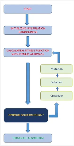
WORKING OF GENATIC ALGORITHM
Genatic algorithm optimisation starts with population initialization
Population is the number of sample data points taken to perform the genetic algorithm operation.
These sample data points undergoes the following three steps:
- Crossover:
It is the process of taking two parents' solutions and producing the child from them.
- Selection:
In this, the parents are selected from the sample data points, the main objective of the selection process is to select the highly fit individuals
- Mutation:
Mutation is carried out to maintain the genetic diversity from one generation of a population of chromosomes to the next.
Fitness function:
Fitness function takes the solution as input and produces the suitability of the solution as the output. This evaluates how close the solution is to the optimal solution of the desired problem.
Syntax for Genetic Algorithm:
(refrence form Matlab help center)
x = ga(fun,nvars,A,b,Aeq,beq,lb,ub)
x = ga(fun,nvars,A,b,Aeq,beq,lb,ub,nonlcon)
x = ga(fun,nvars,A,b,Aeq,beq,lb,ub,nonlcon,options)
x = ga(fun,nvars,A,b,[],[],lb,ub,nonlcon,IntCon)
x = ga(fun,nvars,A,b,[],[],lb,ub,nonlcon,IntCon,options)
[x,fval,exitflag,output] = ga(___)
[x,fval,exitflag,output,population,scores] = ga(___)
here the values means:
x : stores the result from ga optimisation.
ga : used as a function to optimise the "fun" function.
fun: the function that is to be optimised.
nvars: no of variables used in function 'fun'.
A,B : subject to the linear inequalities A*x ≤ b. ga evaluates the matrix product A*x as if x is transposed (A*x').
Aeq,Beq:subject to the linear equalities Aeq*x = beq and A*x ≤ b. (Set A=[] and b=[] if no linear inequalities exist.) ga evaluates the matrix product Aeq*x as if x is transposed (Aeq*x').
lb,ub: is for defining the lower bound and upper bound of the variables in the function 'fun'.
nonlcon : subjects the minimization to the constraints defined in nonlcon. The function nonlcon accepts x and returns vectors C and Ceq, representing the nonlinear inequalities and equalities respectively.
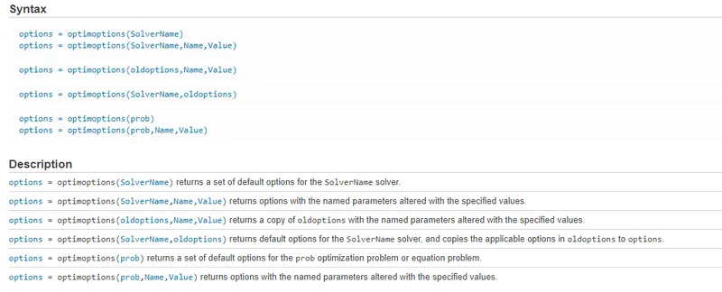
options:minimizes with the default optimization parameters replaced by values in options. (Set nonlcon=[] if no nonlinear constraints exist.) Create options using optimoptions.
options = optimoptions(SolverName)
options = optimoptions(SolverName,Name,Value)
Intcon: requires that the variables listed in IntCon take integer values.
fval: for any previous input arguments, also returns fval, the value of the fitness function at x.
[x,fval,exitflag,output] = ga(___) also returns exitflag, an integer identifying the reason the algorithm terminated, and output, a structure that contains output from each generation and other information about the performance of the algorithm.
[x,fval,exitflag,output,population,scores] = ga(___) also returns a matrix population, whose rows are the final population, and a vector scores, the scores of the final population.
Stopping Criteria Options
Stopping criteria determine what causes the algorithm to terminate. You can specify the following options:
-
MaxGenerations— Specifies the maximum number of iterations for the genetic algorithm to perform. The default is100*numberOfVariables. -
MaxTime— Specifies the maximum time in seconds the genetic algorithm runs before stopping, as measured byticandtoc. This limit is enforced after each iteration, sogacan exceed the limit when an iteration takes substantial time. -
FitnessLimit— The algorithm stops if the best fitness value is less than or equal to the value ofFitnessLimit. Does not apply togamultiobj. MaxStallGenerations— The algorithm stops if the average relative change in the best fitness function value overMaxStallGenerationsis less than or equal toFunctionTolerance. (If theStallTestoption is'geometricWeighted', then the test is for a geometric weighted average relative change.) For a problem with nonlinear constraints,MaxStallGenerationsapplies to the subproblem- For
gamultiobj, if the geometric average of the relative change in the spread of the Pareto solutions overMaxStallGenerationsis less thanFunctionTolerance, and the final spread is smaller than the average spread over the lastMaxStallGenerations, then the algorithm stops. The geometric average coefficient is ½. The spread is a measure of the movement of the Pareto front. -
MaxStallTime— The algorithm stops if there is no improvement in the best fitness value for an interval of time in seconds specified byMaxStallTime, as measured byticandtoc. FunctionTolerance— The algorithm stops if the average relative change in the best fitness function value overMaxStallGenerationsis less than or equal toFunctionTolerance. (If theStallTestoption is'geometricWeighted', then the test is for a geometric weighted average relative change.)- For
gamultiobj, if the geometric average of the relative change in the spread of the Pareto solutions overMaxStallGenerationsis less thanFunctionTolerance, and the final spread is smaller than the average spread over the lastMaxStallGenerations, then the algorithm stops. The geometric average coefficient is ½. The spread is a measure of the movement of the Pareto front. -
ConstraintTolerance— TheConstraintToleranceis not used as stopping criterion. It is used to determine the feasibility with respect to nonlinear constraints. Also,max(sqrt(eps),ConstraintTolerance)determines feasibility with respect to linear constraints.
Where GA is used?
Genetic Algorithms are primarily used in optimization problems of various kinds, but they are frequently used in other application areas as well.
The areas in which Genetic Algorithms are frequently used are listed below.
- Optimization − Genetic Algorithms are most commonly used in optimization problems wherein we have to maximize or minimize a given objective function value under a given set of constraints.
- Economics − GAs are also used to characterize various economic models like the cobweb model, game theory equilibrium resolution, asset pricing, etc.
- Neural Networks − GAs are also used to train neural networks, particularly recurrent neural networks.
- Image Processing − GAs are used for various digital image processing (DIP) tasks as well like dense pixel matching.
Optimization
- Optimisation is a decision making process, it helps to find the best results under a set of prioritized criteria or constraints. It is a procedure which is executed iteratively by comparing various solutions till an optimum or a satisfactory solution is found.
- These include maximizing factors such as productivity, strength, reliability, efficiency, utilization, etc
- Minimum of single and multivariable functions, nonnegative least-squares, roots of nonlinear functions
- Optimizers find the location of a minimum of a nonlinear objective function. You can find a minimum of a function of one variable on a bounded interval using
fminbnd, or a minimum of a function of several variables on an unbounded domain usingfminsearch. Maximize a function by minimizing its negative. - Find a nonnegative solution to a linear least-squares problem using
lsqnonneg. - The equation solver
fzerofinds a real root of a nonlinear scalar function. - Control the output or other aspects of your optimization by setting options using
optimset. - Solve problems and set options using a visual interface with the Optimize Live Editor task.
What are all the techniques available to perform optimisation?
- Deterministic Method: They use specific rules for moving one solution to another. In this technique, the output of the model is fully determined by the parameter values and the initial conditions.
Example:
Stress analysis of the component,this is a deterministic approach since the output results(stress values) fully depend on the initial conditions(loading condition) and the parameter values(force acting on the component and material properties).
- Stochastic Method: These are gaining popularity due to certain properties which deterministic algorithms do not possess.Stochastic models possess some inherent randomness, it is a probabilistic approach.
Example: Varying the water paths from the mountain can vary the regional weather conditions, but the weather condition is not fully dependent on the water paths, hence there will be many statistical predictions to get the predictive model, since the weather condition depends on various factors such as solar distance,latitudinal location, air pressure, etc. Hence it is a predictive model.
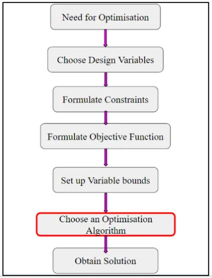
The following is the procedure followed by any optimisation process.
What are variables?
- The parameters which you have to vary during the optimisation process are known as variables.
Example: Design dimensions can be varied to get the minimum stress.
What are Constraints?
- During the optimisation process, your output should not go beyond the certain limits, those are known as constraints.
Example: You can reduce the material used in such a way that the stress should not go beyond the ultimate stress of the material.
What is Objective function?
- Objective function is as simple as a mathematical formulae, which can be a predicted mathematical model that includes all the variables as input.
Example: z=f(x,y) here the output(z) depends on the input variable(x&y).
What are variable bounds?
- The variable bounds are the range of the input variables, that will be varied for every iteration to provide an optimised result.
Example: The design variable (thickness) can be varied in the range between (5-7)mm, to get the minimum stress.
STALAGMITE
A stalagmite is a type of rock formation that rises from the floor of a cave due to the accumulation of material deposited on the floor from ceiling drippings. Stalagmites are typically composed of calcium carbonate, but may consist of lava, mud, peat, pitch, sand, sinter and amberat.
A stalagmite is an upward-growing mound of mineral deposits that have precipitated from water dripping onto the floor of a cave. Most stalagmites have rounded or flattened tips. There are many other types of mineral formations found in caves
Due to its shape we are using the stalagmite as the name for the program
STALAGMITE FUNCTION
A stalagmite function generally refers to the function with which we are generating values over a stalagmite kind of surface for finding out the local and global maxima and minima of that particular given function. 3. For this in Matlab we are using a method called 'Optimization'.
`f(x, y) = f1x*f1y*f2x*f2y`
where f1x, f1y, f2x, f2y
- `f1x = [sin(5.1*pi*x+0.5)]^6`
- `f1y = [sin(5.1*pi*y+0.5)]^6`
- `f2x=exp[-4ln(2)(x-0.0667)^2/(0.64)]`
- `f2y=exp[-4ln(2)(y-0.0667)^2/(0.64)]`
Programe for the stalagmite funtion in MATLAB
function [F] = stalagmitefuntion(input_vector)

x=input_vector(1);
y=input_vector(2);

    f1x = (sin((5.1*pi*x)+0.5))^6;
    f1y = (sin((5.1*pi*y)+0.5))^6;
    f2x = exp((-4*log(2)*(x-0.0667)^2)/0.64);
    f2y = exp((-4*log(2)*(y-0.0667)^2)/0.64);

    F = -(f1x*f1y*f2x*f2y);
end- This is stalagmite function code, we have to call this function to the main programe
Code in MATLAB to optimise the stalagmite function and to find the global maxima of the function.
clear all
close all
clc

x=linspace(0,0.6,100);
y=linspace(0,0.6,100);

[xx,yy]=meshgrid(x,y);

for i=1:length(xx)
    for j=1:length(yy)

        inputs(1)=xx(i,j);
        inputs(2)=yy(i,j);
        F(i,j)=stalagmitefuntion(inputs);
    end
end

num=100;           % Itirations
tic

% Case1 : Statistical Behaviour

for i=1:num
   [inputs,Fopt(i)]=ga(@stalagmitefuntion,2);
    xout(i)=inputs(1);
    yout(i)=inputs(2);
end


casel_time=toc;

figure(1)
subplot(2,1,1)
surfc(xx,yy,-F)
shading interp
hold on
plot3(xout,yout,-Fopt,'marker','*','markersize',5,'markerfacecolor','r')
title('Unbounded Inputs')
subplot(2,1,2)
plot(-Fopt)
xlabel('Iterations')
ylabel('Function Maximum')
tic

%Case2 : Statistical Behaviour with upper bound & lower bound

for i=1:num
    [inputs,Fopt(i)]=ga(@stalagmitefuntion,2,[],[],[],[],[0;0],[0.6;0.6],[],[]);
    xout(i)=inputs(1);
    yout(i)=inputs(2);
end

case2_time=toc;

figure(2)
subplot(2,1,1)
surfc(x,y,-F)
shading interp
hold on
plot3(xout,yout,-Fopt,'marker','*','markersize',5,'markerfacecolor','g')
title('Bounded Inputs')
subplot(2,1,2)
plot(-Fopt)
xlabel('Iterations')
ylabel('Function Maximum')
tic

%Case3 : Increasing population

options=optimoptions('ga');
options=optimoptions(options,'populationsize',300);

for i=1:num
[inputs,Fopt(i)]=ga(@stalagmitefuntion,2,[],[],[],[],[0;0],[0.6;0.6],[],[],options);
xout(i)=inputs(1);
yout(i)=inputs(2);
end

case3_time=toc;

figure(3)
subplot(2,1,1)
surfc(x,y,-F)
shading interp
hold on
plot3(xout,yout,-Fopt,'marker','*','markersize',5,'markerfacecolor','b')
title('Bounded Inputs with Increased Population size')
subplot(2,1,2)
plot(-Fopt)
xlabel('Iterations')
ylabel('Function Maximum')
CODE EXPLINATION
- Creating a X and Y 1D vector 100 values b/w 0 to 0.6
- And by using the meshgrid we are creating the 2D vector where XX and YY
- By creating the for loop for I and J to the length of XX and YY
- inputs(1)=xx(i,j);
inputs(2)=yy(i,j); - And then we illbe calling the stalagmite functionand inserting the inputs in that
- Three cases
Case1 : Statistical Behaviour
Case2 : Statistical Behaviour with upper bound & lower bound
Case3 : Increasing population
Case1 : Statistical Behaviour
-
To study the behaviour of the genetic algorithm without applying any condition to the optimisation process.
-
Here we have to find out the global maxima so that we will be giving the negitive sign for the function
-
Tic and toc command is used to get the study time taken for the ga to run
-
For loop is used to run the ga for 100 times
-
Through ga we will be calling the stalagmitefunction and giving the no of variables used in function is 2
-
Outputs are
-
xout(i)=inputs(1);
yout(i)=inputs(2); - And plotting graph using plot3 command
plot3( plots coordinates in 3-D space.X,Y,Z)
To plot a set of coordinates connected by line segments, specify X, Y, and Z as vectors of the same length.
To plot multiple sets of coordinates on the same set of axes, specify at least one of X, Y, or Z as a matrix and the others as vectors.
- By using subplot command we will be plotting the graphs in one window only
CODE FOR THE CASE 1
% Case1 : Statistical Behaviour

for i=1:num
   [inputs,Fopt(i)]=ga(@stalagmitefuntion,2);
    xout(i)=inputs(1);
    yout(i)=inputs(2);
end


casel_time=toc;

figure(1)
subplot(2,1,1)
surfc(xx,yy,-F)
shading interp
hold on
plot3(xout,yout,-Fopt,'marker','*','markersize',5,'markerfacecolor','r')
title('Unbounded Inputs')
subplot(2,1,2)
plot(-Fopt)
xlabel('Iterations')
ylabel('Function Maximum')
tic- Time taken to run the case 1 is 7.7559 s
- Below plot shows the case 1 results
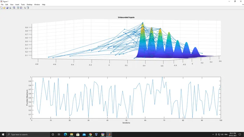
- Result is like this because we have not given the bounds that should be limit in the x and y values
Case2 : Statistical Behaviour with upper bound & lower bound
- ga is defined with function name ,no of variables and also boundation for the optimisation is set to 0 to 0.6
CODE FOR THE CASE 2
%Case2 : Statistical Behaviour with upper bound & lower bound

for i=1:num
    [inputs,Fopt(i)]=ga(@stalagmitefuntion,2,[],[],[],[],[0;0],[0.6;0.6],[],[]);
    xout(i)=inputs(1);
    yout(i)=inputs(2);
end

case2_time=toc;

figure(2)
subplot(2,1,1)
surfc(x,y,-F)
shading interp
hold on
plot3(xout,yout,-Fopt,'marker','*','markersize',5,'markerfacecolor','g')
title('Bounded Inputs')
subplot(2,1,2)
plot(-Fopt)
xlabel('Iterations')
ylabel('Function Maximum')
tic- Result plots are shown below
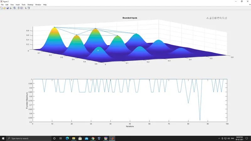
- Time taken to run code is 10.5900 s
- Here we are getting the some of maximum values for the given inputs but we need global maxima
Case3 : Increasing population
- In this case we are going to change the inputs
- We are going to increase the population number by using the option command in the ga
- Increasing the population to 300 will makes the function to run longer and calculate with more values gives the optimum value
CODE FOR THE CASE 3
%Case3 : Increasing population

options=optimoptions('ga');
options=optimoptions(options,'populationsize',300);

for i=1:num
[inputs,Fopt(i)]=ga(@stalagmitefuntion,2,[],[],[],[],[0;0],[0.6;0.6],[],[],options);
xout(i)=inputs(1);
yout(i)=inputs(2);
end

case3_time=toc;

figure(3)
subplot(2,1,1)
surfc(x,y,-F)
shading interp
hold on
plot3(xout,yout,-Fopt,'marker','*','markersize',5,'markerfacecolor','b')
title('Bounded Inputs with Increased Population size')
subplot(2,1,2)
plot(-Fopt)
xlabel('Iterations')
ylabel('Function Maximum')- Result plots are shown below
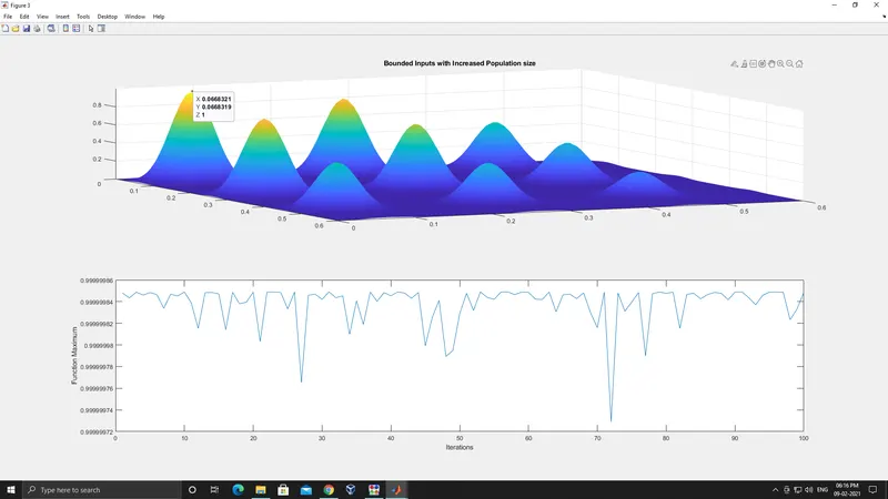
- Time taken to run code is 46.8178 s
- Here we are getting the global maxima
CONCLUSION
we can see that the result of the optmisation is improved while changing the condition for the optmisation of the function like
- boundry conditions for the optimisation process
- increasing the population size
But while increasing the condition for optimisation process through ga the time required fro the optimisation also increased a lot.
so we can get the most optimum results form optimisation but the time required for the optimisation is also going to increase with it.
ERRORS FACED
- Always look whether we are giving correct sign or not one example is shown below
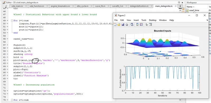
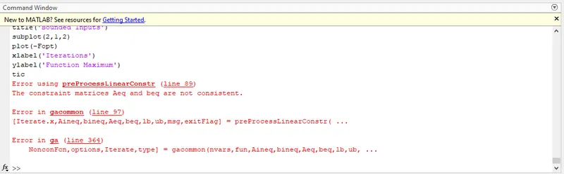
- Number of inputs should be equal in the ga command or else its going to throw a error as shown