Week 4 - Genetic Algorithm

AIM:

To create a algorithm that will search for the maximum value a function can yield and optimize it

OBJECTIVE:

1) Create a fitness function that will yield the result

2) Use genetic algorithm to search for the maximum value of the fitness function and hence the function gets optimized.

GENETIC ALGORITHM:

As said in the video too, a Brute force search technique is tedious and time ingesting, therefore there are lot of search heuristics and optimization techniques available to ease the function optimization. One efficient proven is genetic algorithm rudimented from Darwinism.

A genetic algorithm simulates, mimics the samen idea as human evolution " Survival of the fittest ". Some detailed steps are as follows:
1) The algorithm chooses random population sample, i.e data or information or functional yields initially.

2)Then the algorithm iterates the value against the fitness function as parent are being transmitted to the next generation

3) With every iteration it will progress by reducing its population size. Calculate fitness for the new population.

4) Then at one point the algorithm will converge to a point, the optimum point, maxima. Survival of the fittest.

So why genetic algorithm?

Concisely, robustness. Among the other traditional optimization or gradient based methods, genetic algorithm when the function has wider local maxima or minima, the function oscillates then genetic algorithm proves much more efficient. The paramount advantage is that with the continuous iteration and the random population sample selection, regardless of the initial points or the local optimised value the global optimization will converge at the global optimum.

ga:

Matlab has an inbuilt function to generate the code for genetic algorithm that can be accessed with the keyword "ga". The genetic algorithm in matlab can also be given with function's mathematical attributes like the linear equalities, inequalities, bounds, population size etc. The syntax explained here as:

x = ga(@fitness function, number of variables)

The basic syntax mentioned above requires the fitness function where the values are tested against has to be mentioned and the number of variables in the generation process.

x = ga(@fitness function, number of variables,Aineq,Bineq,Aeq,Beq)

This version of the syntax will compute for the inequalities and the equalities respectively. When the function has the linear models then this can be carried out to the search heuristic.

x = ga(@fitness function, number of variables,Aineq,Bineq,Aeq,Beq,Lower bounds, Upper bounds)

This syntax quiet came in handy while doing this project as the bounds were really helpful in scrutinizing and shortening the output yield.

Generally, the upper bounds and lower bounds are specified so that the value of the 'x' is found in this range. This also helps in avoiding the function to converge to the local optimum rather than the global optimum.

x = ga(@fitness function, number of variables,Aineq,Bineq,Aeq,Beq,Lower bounds, Upper bounds,options)

Another vital option is the 'options' in the syntax. Like we can specify to modify the search algorithm for instance mentioning the initial point of the search space, population size etc.

CODE STRUCTURE:

1. INPUTS

Using linspace command we are creating any two arbitrary arrays.

% Creating values for x and y
x = linspace(0,0.6,150);
y = linspace(0,0.6,150);

With the help of meshgrid we are making the array above created as square matrix so that the calculation against the fitness function is carried out with each and every values against it.

% Making the above array as square matrix
[xx, yy] = meshgrid(x,y);

Specify the iterations has to be carried out, biologically the generations.

% Iterations to be carried out
num_cases = 50;

2. EVALUATION

Now, we are using the values created and evaluating it against the fitness function. This will generate the population that needs to searched and optimised.

 Evaluating the values against the function
for i = 1:length(xx)
     for j =  1: length(yy)
         input_vector(1) = xx(i,j);
         input_vector(2)= yy(i,j);
         f(i,j) =  stalagmite(input_vector);       
     end
end

The fitness function which just has some mathematical calculation. Once the computation is made then the values are stored and returned to the 'f', the output variable.

% Fitness function

function [ f ] = stalagmite(input_vector)
% Computation
f1 = (sin(5.1.*pi.*input_vector(1) + 0.5)).^6;
f2 = (sin(5.1.*pi.*input_vector(2) + 0.5)).^6;
f3 = exp(-4.*log(2) .* ((input_vector(1) - 0.0667)^2)/0.64);
f4 = exp(-4.*log(2) .* ((input_vector(2) - 0.0667)^2)/0.64);
f = -(f1.*f2.*f3.*f4); % Maximum value
end

3. OPTIMIZATION:

And now we are searching for the optimum value that are tested against the fitness function. And then plotting the same values using 3-D plot will yield us value but the optimum values of the function are scattered and are difficult to conclude or converge. Also there are chances that the code might converge to local optimum value with such a wider range.

% Initial normal study
for i = 1 : num_cases
    [inputs, f_max(i)] = ga(@stalagmite,2);
    xval(i) = inputs(1);
    yval(i) = inputs(2);
end

Hence, to overcome the above mentioned crisis we are specifying the output search space with boundaries i.e we are giving commands so that the value of the optimum lies within that specified range.

This we are specifying as discussed in the syntax explanation of ga above.

 Optimizing by binding the 'x' value within certain limit
for i = 1 : num_cases
    [inputs, f_max(i)] = ga(@stalagmite,2,[],[],[],[],[0;0],[1;1]);
    xval(i) = inputs(1);
    yval(i) = inputs(2);
end

Once this is generated we could see a narrowing of the output values but still not the optimum or desired value. So, we are specifying the search space with some user defined options or characteristics.

Here, we are specifying the population size of the search space. This will narrow down the results further down but the cons is that the time elapsed might be longer than the normal search heuristics.

% Specifying the options for the genetic algorithm
options  = optimoptions('ga');
options = optimoptions(options,'PopulationSize',300);

% Bounded and specified optimization
for i = 1 : num_cases
    [inputs, f_max(i)] = ga(@stalagmite,2,[],[],[],[],[0;0],[1;1],[],[],options);
    xval(i) = inputs(1);
    yval(i) = inputs(2);
end

So how to deal with the time elapsing?

1) One way would be to pre allocate the variables, the variables inside the loop are pre allocated with larger values so that the values are not to be re allocated for every iteration rather it it already done.

2) But the above method yields negligible results, a rather better approach would be to start the search space with genetic algorithm and use a traditional search optimization when there is certainity for the optimized range, hybrid optimization..

TIME ELAPSED:

We are using tic and toc in built commands to calculate the time elapsed for every iterations.

PLOTTING:

We are creating 3 separate figures to compare our study. Each figure has subplots to have multiple graphs in the same window.

Then we are using the surface command to create a surface of the optimum function. This will produce a 3- dimensional surface plot of the variables specified.

Then we are plotting another 3-D plot with a marker that will give us the points were the function is ranging between

And finally we are plotting the optimum value against every iteration. This will give us the range of the converging point so can be used to narrow down.

The hold on, labels and title are usual commands used.

figure(1)
subplot(2,1,1) % Two plots in the same figure
hold on
surfc(x,y,-f) % surface plot
shading interp
plot3(xval,yval,-f_max,'marker','o','markersize',5,'markerfacecolor','r')
subplot(2,1,2)
plot(f_max)
xlabel('Number of Iterations')
ylabel('Maxima of the function')

CODE:

clear all
close all
clc
% Stalagmite
% Maxima of the function

% Creating values for x and y
x = linspace(0,0.6,150);
y = linspace(0,0.6,150);

% Making the above array as square matrix
[xx, yy] = meshgrid(x,y);

% Iterations to be carried out
num_cases = 50;

% Evaluating the values against the function
for i = 1:length(xx)
     for j =  1: length(yy)
         input_vector(1) = xx(i,j);
         input_vector(2)= yy(i,j);
         f(i,j) =  stalagmite(input_vector);       
     end
end

% Initial normal study
tic
for i = 1 : num_cases
    [inputs, f_max(i)] = ga(@stalagmite,2);
    xval(i) = inputs(1);
    yval(i) = inputs(2);
end
study1_time = toc;  % Calculating time elapsed for the study

rng default

% Plotting
figure(1)
subplot(2,1,1) % Two plots in the same figure
hold on
surfc(x,y,-f) % surface plot
shading interp
title(' Ideal search and optimization')
plot3(xval,yval,-f_max,'marker','o','markersize',5,'markerfacecolor','r')
subplot(2,1,2)
plot(f_max)
title(' Optimum value of the function')
xlabel('Number of Iterations')
ylabel('Maxima of the function')

% Optimizing by binding the 'x' value within certain limit
tic
for i = 1 : num_cases
    [inputs, f_max(i)] = ga(@stalagmite,2,[],[],[],[],[0;0],[1;1]);
    xval(i) = inputs(1);
    yval(i) = inputs(2);
end
study2_time = toc;
rng default
figure(2)
subplot(2,1,1)
hold on
surfc(x,y,-f)
shading interp
title(' Searching and binding the optimized value')
plot3(xval,yval,-f_max,'marker','o','markersize',5,'markerfacecolor','r')
subplot(2,1,2)
plot(f_max)
title(' Optimum value of the function')
xlabel('Number of Iterations')
ylabel('Maxima of the function')

% Specifying the options for the genetic algorithm
options  = optimoptions('ga');
options = optimoptions(options,'PopulationSize',300);

% Bounded and specified optimization
tic
for i = 1 : num_cases
    [inputs, f_max(i)] = ga(@stalagmite,2,[],[],[],[],[0;0],[1;1],[],[],options);
    xval(i) = inputs(1);
    yval(i) = inputs(2);
end
study3_time = toc;
rng default
figure(3)
subplot(2,1,1)
hold on
surfc(x,y,-f)
shading interp
title('Bounded and specified optimization')
plot3(xval,yval,-f_max,'marker','o','markersize',5,'markerfacecolor','r')
subplot(2,1,2)
plot(f_max)
title(' Optimum value of the function')
xlabel('Number of Iterations')
ylabel('Maxima of the function')

CONSTANT OUTPUT:

The code when ran for each time will give and produce different values of output at each execution. To avoid this and make the search and optimization more certainable, there is in-built function used.

This is because the genetic algorithm searches and picks random number of 'n' sized population and with every varying execution this is varied and hence the output.

rng default

This will control the random generation of the population and then the defaults the population during the iterations such that the values are not changed but remains the same after different execution.

OUTPUT:

Now, we got to compare the outputs of the above three search and optimization methods.

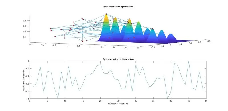
As we can see in the above image, the markers help to identify the converging points of the search space at every iteration. This is really a wider variation and also the optimum value range is very high and hence not desired.

BOUNDED OPTIMIZATION

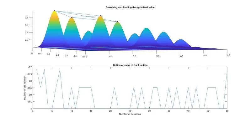
The bouned search reduces the predicted space value to 4 points. This is very far narrowed from the above results but still this can be reduced to a more narrow range.

BOUNDED AND SPECIFIED OPTIMIZATION:

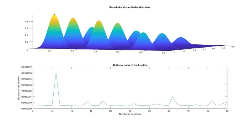
With all the binding of the outputs and specifying the population size we can see that the predicted value lies in only one of the peak value and also the optimum value lies within a very negligible range now.

TIME ELAPSED:

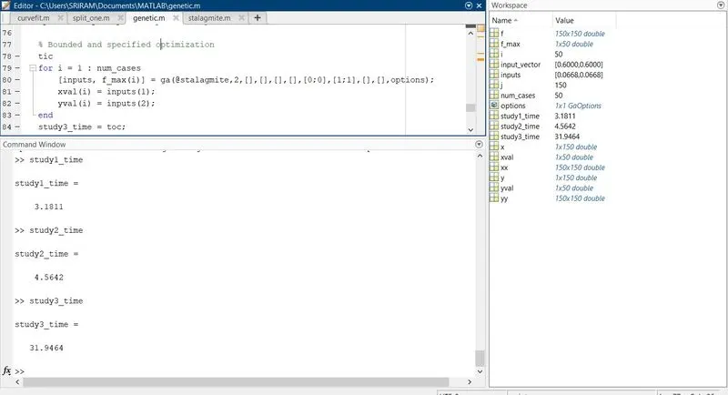
The time ingested for all the three iterations are shown below. As we could see the more the accurate and narrower the range and the optimum value is the time is relatively higher.

ERRORS:

While programming minor and impulsive errors were made which were rectified then and there.

But a logical error made was when I didn't store the output value of the optimized values in the for loop as array rather I stored them as variable.

CONCLUSION:
The genetic algorithm when made with proper bounding of the outut range, making the search space narrower and more specific options will yield very efficient and potential results.