Week 3 - Solving second order ODEs

AIM:
To solve a second order differential equation, observe and record the behaviour of the system having the second order differential transient behaviour.

OBJECTIVE:
1) To trace the velocity and angular displacement of a simple pendulum using its equation of motion

2) Concatenate the angular displacements and position w.r.t time of the pendulum and create an animation

SIMPLE PENDULUM:

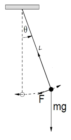
The simple pendulum consists of a bob and a string that has periodic oscillatiory motion when a initial force is imparted. When a simple pendulum is displaced from its equilibirum position, there will be a restoring force that moves the pendulum back towards its equilibrium position.

GOVERNING EQUATION:

The general governing equation of a simple pendulum is as follows

`(d^2theta)/(dt^2) + b/m*(d theta)/dt + g/l*sin theta`

Here, 'b' is the damping co-efficient of the oscillation,

`m' is the mass of the bob,

'g' is acceleration due to gravity,`

`L' is the length of the suspended string, assumed massless, and

`theta` is the angular displacement.

CODE STRUCTURE:

1.INPUTS

The input parameters required are given as per specified and they are given with their respective units.

% INPUTS

% damping coefficient
b = 0.05;
% acceleration due to gravity in m/s^2
g = 9.81;
% length of the massless string in 'm'
l = 1;
% mass of the bob in 'kg'
m = 1;

The time interval is also given, since the displacement and velocity are specified with respect to time, here we are creating between 0 to 20 seconds with a discrete 500 values. For creation of this time array we use linspace command.

% time span for the motion of pendulum
t_span = linspace(0,20,500);

The pendulum has to be given a initial velocity to set its motion. Here we are giving them input as two diferent columns angular displacement and velocity in a single array and storing the same.

% Initial angular displacement and velocity of the pendulum
theta_0 =  [0;3];

2. DIFFERENTIATING

For the differentiation of the equation we are using an inbuilt function named "ode45". The syntax of the function and its inputs are as follows.

A) Initially, the inbuilt function ode45 and followed by it we are giving the dependent and independent variables of the equation, time and angular displacement here, since the equation is governed with respect to time

ode45(@(t,theta)

B) And then we are calling the function odefunc where the coding for second order differential is explained below.

odefunc(t,theta,b,g,l,m)

C)Now we need to pass the individual values of the governing variables that we assigned initially. This will pass the values for every iteration and then the respective calculation is carried out

t_span,theta_0

3. SOLVING THE SECOND ODE:

To solve the second differential of the equation, we are assigning `theta = theta1`. And then differentiate for the first time. Then we are assigning this first order differential as `theta2`.Differentiating this again will give the second order of the same equation i.e `(d^2theta)/dt^2`

And then finally store them to an array named dtheta, the values of dheta1 and dtheta2.

function dtheta = odefunc(t,theta,b,g,l,m)

theta1 = theta(1);
theta2 = theta(2);
dtheta1 = theta2;
dtheta2 = ((-b/m)*theta2) - (g/l*sin(theta1));
dtheta = [dtheta1 ; dtheta2];

end

PLOTTING THE GRAPHICAL REPRESNTATION:

A) DISPLACEMENT, VELOCITY vs TIME

Now we are plotting the calculated values. Asusual the plot command is used and the curve specifications are mentioned. Additionally we are using hold on and hold off commands because there are more than one graph we are plotting in the same figure and hence this will retain both the curves in the graph. Labels are given and the curve specifications are also mentioned using the respective commands.

% plotting the angular displacement and velocity
figure(1)
hold on
plot(t,results(:,1),'color','r')
plot(t,results(:,2),'color','b')
hold off
xlabel('Time in s')
ylabel('Angular displacement in rad/sec, Velocity in m/s')
legend('Angular Displacement','Velocity')

B) PENDULUM TRACE

The pendulum position calculated earlier with respect to the time is now has to be plotted to create its motion. For this again we are using the same plot command and then a new figure.

A) The x1 and y1 values for the pendulum are located using the sine and cosine terms. Then they are used to plot the positions.

 x0 = 0;
 y0 = 0;

x1 = l*sin(results(i));
y1 = -(l*cos(results(i)));
plot([x0 x1] , [y0 y1], 'linewidth',3,'color',[0.753 0.753 0.753]

B) Now, we are creating simple representation of the pendulum pivot point for which we are creating a line with width to represent like a bar.

plot([-1 1],[0 0],'linewidth', 5,'color',[0,0,0])

C) Finally for the bob, we are using the marker tool and plotting it at the other end, the oscillating, to give a pictorial representation of the bob.

plot(x1,y1,'marker','o','markersize',18,'markerfacecolor','b')

D) The hold on and hold off commands play the vital role as we already know matlab only plots the recent plot command negelecting the earlier ones. So, there is a necessity to use them. Moreover using them, their location is also another crucial aspect. The massless string and the bob are those in motion and hence we are using the hold on and hold off for the command starting and ending respectively. With the hold on command the pivot bar is not obsolete.

plot([-1 1],[0 0],'linewidth', 5,'color',[0,0,0])
    
    hold on
    plot(x1,y1,'marker','o','markersize',18,'markerfacecolor','b')
        
    plot([x0 x1] , [y0 y1], 'linewidth',3,'color',[0.753 0.753 0.753])
    hold off

ANIMATION

The objective is create an animation of the motion of the pendulum. For this we are using the counter variable and for loop which will iterate for each and every value of the time and displacement. Then the each position of the plot is gathered using the getframe(gcf) command. And then with the counter variable these are concatenated. We are giving a minuscule pause between the frames. In the "for" command, we are actually accessing the first column of the results matrix which is angular displacement.

ct = 1;
figure(2)
for i = 1:length(results(:,1))

 M(ct) =  getframe(gcf);
    pause(0.0000003);
    ct=ct+1;

For the movie creation with the concatenated frames we are using the inbuilt function as follows:

% movie creation
videofile = VideoWriter('pendulum.avi','Uncompressed AVI');
open(videofile);
writeVideo(videofile,M);
close(videofile);

RESULTS:

The displacement, velocity vs time graph yields as follows for the given input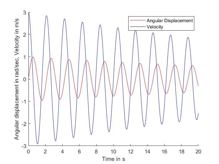

The animated video file is here

ERRORS:

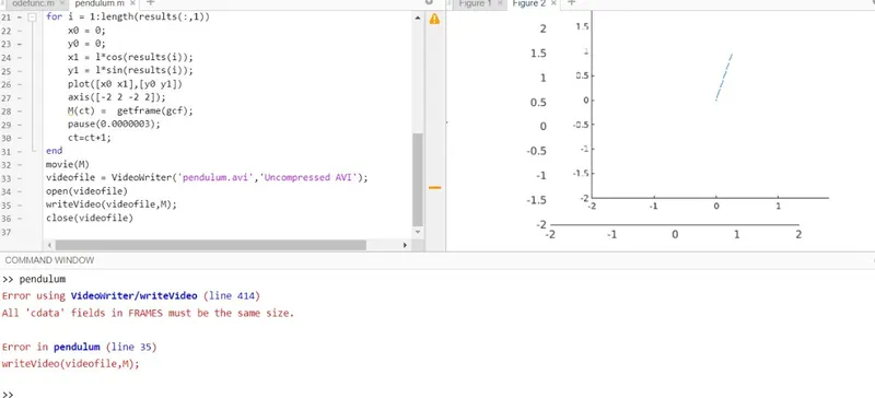
While using the matlab online I did face the same error as earlier and then during the matlab application solve the error didn't appear.

CONCLUSION:

The same graph and the animation video is created and the values are analysed.