Project 2 - Rankine cycle Simulator

AIM:
To compute a program that simultes the rankine cycle based on the user inlet conditions.

OBJECTIVE:
1) To get the input from the user as the independent variables and then find out the properties at the state points.

2) To plot the temperature-entropy and enathlpy-entropy diagram for the above calculated state points.

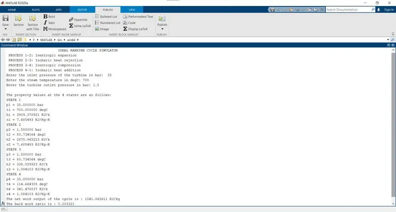
3) Also calculate the net work output of the cycle and the back work ratio i.e the ratio of the turbine to the pump work.

RANKINE CYCLE:

One of the most idealized thermodynamic cycle that describes for the heat engines, steam turbines etc. In a Rankine cycle there is a operating fluid that circulates into the system. This is one of the most idealized cycle used to maximize the mechanical work output. Before into the process, practically, There are four core components in a Rankine cycle that are as follows:

1. Steam generator typically a boiler where the working fluid is heated above its saturated temperature, superheated state. This process is carried out keeping the pressure constant.

2. Turbine is where the energy conversion takes place. The steam from the boiler flows into it and the turbine extracts the pressurized energy and converts it into the mechanical work.

3.Condenser operates at a constant pressure where heat is released into the environment, compressing the state of the fluid back down to a liquid-gas mixture, that is mostly liquid. This state is otherwise known as “saturated liquid.”

4.Pump then pressurizes the saturated liquid back up to the pressure of the turbine by bringing work back into the system, turning to a highly pressurized liquid.

Now the process is as follows:
1-2: Isobaric heat addition, is where the fluid is heated to the superheated state without changing its pressure energy.

2-3: Isentropic expansion, when the fluid enters the turbine it expands resulting a pressure drop as the turbine converts them to the mechanical work.

3-4: Isobaric heat rejection: Now, before the process occurs again the steam phase has to be changed which is carried out by the condenser. Here, the fluid becomes goes into the liquid state.

4-1: Isentropic compression process includes a pump where the fluid from the condenser is compressed to maintain the pressure at the inlet of the turbine.

WORK OUTPUT:

The primary function is generate the work from the fluid, therefore in finding the work output of the cycle, we need to find the turbine work done and also the pump work. The key difference is that on the turbine work is extracted and in the pump work is exerted. Also the back work ratio gives a picture about the work ratio in the cycle as a part of the turbine work is used to compress the fluid in the pump or the compressor.

The equation for finding the work in the turbine and the pump are given as:

`Wtau = h1- h4;`

`Wrho = h3-h4;`

CODE STRUCTURE:

INPUT:

The pressure at the inlet of of the turbine and the condenser , temperature at the outlet of the turbine are being given as input from the user. These are the independent properties that are used to find other state properties.

% Initial conditions input from the user
p1 = input('\nEnter the inlet pressure of the turbine in bar:  ');
t1 = input('Enter the steam temperature in degC: ');
p2 = input('Enter the turbine outlet pressure in bar: ');

Once the independent properties are from the user, the rest is to calculate the state properties. The properties at each state are as follows:

STATE 1:

The enthalpy and entropy at the state 1 is extracted from the XSteam file as follows:

% extracting the enthalpy and entropy at state 1 from the file 
h1 =  XSteam('h_pT',p1,t1);
s1 =  XSteam('s_pT',p1,t1);

STATE 2:

Since at the turbine there is isentropic expansion, the temperature change can be calculated as follows using the isentropic equation.

t2 = t1*((p2/p1)^(gamma-1/gamma)); % isentropic equation

Now, since the pressure and temperature of the state points are known, we can calculate rest of the properties. As said about the isentropic expansion,

s2 = s1 % Due to isentropic expansion

The fluid phase changes and hence the steam fraction i.e the dryness fraction has also to be considered. Now the enthalpy and entropy are calculated as:

hf2 = XSteam('hL_p',p2); % enthalpy at liquid state
hg2 = XSteam('hV_p',p2); % enthalpy at gaseous state
sf2 = XSteam('sL_p',p2); % entropy at liquid state
sg2 = XSteam('sV_p',p2); % entropy at gaseous state
x2 = ((s2-sf2)/(sg2-sf2)); % dryness fraction

Enthalpy and entropy at the liquid and gaseous state are extracted from the steam function.

h2 = hf2 + (x2*(hg2 - hf2)); % enthalpy at the outlet of turbine

STATE 3:

At the condenser, only the phase change of the liquid take place hence the pressure remains constant as the turbine outlet pressure.

p3 = p2; % Isobaric heat rejection
t3 = t2;

Thus from these two properties the enthalpy, entropy and the specific entropy of the state are obtained from the file.

% enthalpy, entropy and specific volume from the file
h3 = XSteam('hL_T',t3); 
s3 = XSteam('sL_T',t3); 
v3 = XSteam('vL_T',t3);

STATE 4:

Since in the pump there is only isentropic compression takes place the entropy remains constant as in the previous state. Also the pressure at the outlet of the pump is generated upto the pressure at the inlet of the turbine. Hence that property is also known now.

s4 = s3; % isentropic compression
p4 = p1; % constant pressure at the inlet and outlet of the turbine

Then the specific volume and the specific pressure are extracted from the steam file as follows:

cp4 = XSteam('Cp_ps',p4,s4); % constant pressure at state4
cv4 = XSteam('Cv_ps',p4,s4); % constant volume at state4

Now after that the isentropic constant is calculated and then the temperature at state 4 is found out. Once then the enthalpy at the point 4 is also calculated.

k = cp4/cv4; % constant
t4 = t3/((p3/p4)^(k-1)/k); % isentropic process
h4 = h3 + v3*(p4-p3)*100; % enthalpy at state 4

The fluid as said gets superheated and hence those property values are also has to taken into consideration.

% superheated state from the boiler
t6 = XSteam('Tsat_p',p1);
s5 = XSteam('sL_p',p1);
s6 = XSteam('sV_p',p1);
h5 = XSteam('hL_p',p1);
h6 = XSteam('hV_p',p1);
t5 = t6;

WORK DONE:

Described as above the work done by the turbine, pump and the back work ratio are calculated.

% calculation of work done and back work ratio
wt = h1 - h2; % turbine work
wp = h3 - h4; % pump work
net_work = wt - wp; % Net work output in the cycle
bwr = -(wp/wt); % back work ratio

PLOTTING:

Once all the state properties required are found out the graph can be plotted. The graph requires the saturation curve too and hence we are creating such a curve using the temperature vs entropy at these temperature points at both liquid and gaseous state.

%Creating the array values for saturation curve
temp_range = linspace(0,2000,2000); % for the saturation curve
for i = 1:length(temp_range)
    sf(i) = XSteam('sL_T',temp_range(i)); % Saturated liquid entropy
    sg(i) = XSteam('sV_T',temp_range(i)); % Saturated gas entropy
    hf(i) = XSteam('hL_T',temp_range(i)); % saturated liquid enthalpy
    hg(i) = XSteam('hV_T',temp_range(i)); % Saturated gas enthalpy
end

Then, the saturation curve is plotted as follows:

% Saturation curve
plot(sf,temp_range,'linestyle','- -','color','r','linewidth',1);
plot(sg,temp_range,'linestyle','- -','color','r','linewidth',1);

And finally the state values are plotted as follows:

% process 1 - 2
plot([s1 s2], [t1 t2],'color',[0 0 0],'linewidth',2);
text(s1,t1+0.25,'1'); % indicating the path
% process 2 - 3
plot([s2 s3], [t2 t3],'color',[0 0 0],'linewidth',2);
text(s2+0.25,t2+0.25,'2');
% process 3 - 4
plot([s3 s4], [t3 t4],'color',[0 0 0],'linewidth',2);
text(s3-0.25,t3,'3')
% process 4 - 1
plot([s4 s5], [t4 t5],'color',[0 0 0],'linewidth',2);
text(s4-0.25,t4,'4')
% superheated state
plot([s5 s6], [t5 t6],'color',[0 0 0],'linewidth',2);
plot([s6 s1],[t6 t1],'color',[0 0 0],'linewidth',2);

The function 'text' is used to input text into the graph, the state points.

Then the graph detailings are made.

% Graph plot detailing
xlabel('Entropy')
ylabel('Temperature')
grid minor
legend('Saturation curve','Location','northwest');
title('Rankine cycle process, Temperature,t vs Entropy,s')
% process name specification
set(gtext('Isentropic expansion'),'Rotation',90);
set(gtext('Isobaric heat rejection'));
set(gtext('Isentropic compression'),'Rotation',90);
set(gtext('Isobaric heat addition'),'Rotation',70);

The 'gtext' is used to insert text into the graph at desired locations and the set function is used for the orientation of the text.

The same being carried out for enthalpy and entropy graph plot.

figure(2)
hold on
plot(sf,hf,'linestyle','- -','color','r','linewidth',1);
plot(sg,hg,'linestyle','- -','color','r','linewidth',1);
plot([s1 s2], [h1 h2],'color',[0 0 0],'linewidth',2);
text(s1,h1+0.25,'1');
plot([s2 s3], [h2 h3],'color',[0 0 0],'linewidth',2);
text(s2,h2+0.25,'2');
plot([s3 s4], [h3 h4],'color',[0 0 0],'linewidth',2);
text(s3-0.25,h3+0.25,'4');
plot([s4 s1], [h4 h1],'color',[0 0 0],'linewidth',2);
text(s4+0.25,h4-0.25,'3');
xlabel('Entropy')
ylabel('Enthalpy')
grid minor
legend('Saturation curve','Location','northwest');
title('Rankine cycle process, Entropy, s vs Enthalpy,h')

OUTPUT DISPLAY:

The calculated state properties and the work done are displayed in the command window using the fprintf function.

% output generation
fprintf('\nThe property values at the 4 states are as follows: \n' );
fprintf('STATE 1\n')
fprintf('p1 = %f bar\nt1 = %f degC\nh1 = %f KJ/k\ns1 = %f KJ/Kg-K\n',p1,t1,h1,s1);
fprintf('STATE 2\n')
fprintf('p2 = %f bar\nt2 = %f degC\nh2 = %f KJ/k\ns2 = %f KJ/Kg-K\n',p2,t2,h2,s2);
fprintf('STATE 3\n')
fprintf('p3 = %f bar\nt3 = %f degC\nh3 = %f KJ/k\ns3 = %f KJ/Kg-K\n',p3,t3,h3,s3);
fprintf('STATE 4\n')
fprintf('p4 = %f bar\nt4 = %f degC\nh4 = %f KJ/k\ns4 = %f KJ/Kg-K\n',p4,t4,h4,s4);
fprintf('The net work output of the cycle is : %f KJ/kg\n',net_work);
fprintf('The back work ratio is : %f \n',bwr);

OUTPUT:

The temperature vs entropy curve is as follows: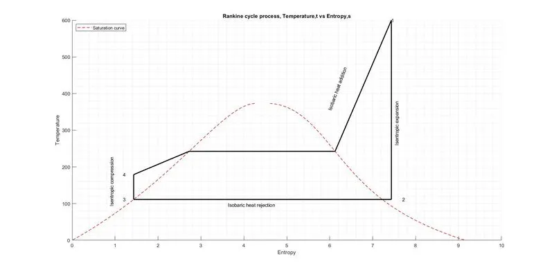

Enthalpy vs entropy curve:

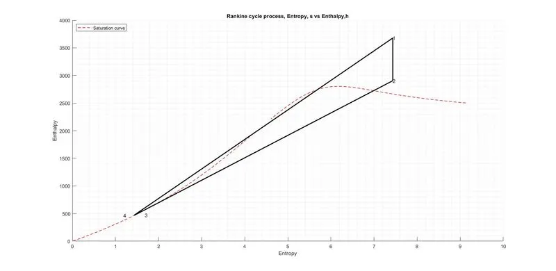
The output command window:

ERRORS:

The compilation was quite smooth and no logical or syntax errors were faced.

CONCLUSION:

The rankine cycle is simulated and the graphical curves are plotted based on the user input.

REFERENCES:

https://www.instructables.com/Simple-Rankine-Cycle-Thermodynamics/

https://www.youtube.com/watch?v=lhilSmE2Ee0