Project 1 - Parsing NASA thermodynamic data

AIM:

To be able to parse the raw data from a file and then manipulate the given data to produce desired results and output.

OBJECTIVE:
1) Initially, break down the parsed file into its components.

2) Segregate the computational data and the header files, other meaningful data that would be desired.

3) Compute the specific heat, enthalpy, entropy at the given local temperature range and then plot, save the output to its species folder which should be auto-generated.

4) Calculate the molecular weight of the species.

5) Make coding to calcualte the above results exclusively to the user given input.

PARSING:
As the word synonyms in English, parsing means to resolve the components it holds, recite them to their respective roles in a way it makes meaningful information.

NASA THERMODYNAMIC DATA:

NASA came up with such a raw data of information that holds the values required to calculate the thermodynamic properties of more than 1000 species. Now we are working on manipulating the data on a typifying level of species. A sample picture of the data is shown below.

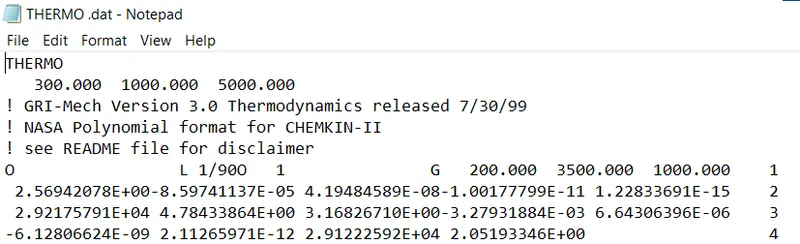
The THERMO.DAT file contains the substantial information to calculate the specific heat, enthalpy, entropy of the respective species for their desired local temperature range.

CODE STRUCTURE:

FILE OPENING:

Initially, the file with the species data has to be loaded into the matlab for parsing the data. This can be done with the "fopen" function as follows:

% opening the NASA FILE
fid = fopen('THERMO','r');

DATA EXTRACTION:

From the file the data has to be extracted and has to be segregated and stored as meaningful information so as to proceed for the calculation. This initial parsing of the raw data can be carried out by a method involving a built in function known as regular expression abbreviated in MATLAB as "regexp".

% Splitting the file by each line
line_split = regexp(fileread('THERMO'), '\n','split');

The function syntax goes, selecting the file to be parsed on, choosing the delimiter, new line in our code and then determing the delimiter function. Here we are splitting them and then storing them. While storing them they are being stored as charcters in a cell array which function slight different from the normal matrix array, also explained in the later part.

DATA SEGREGATION:

1) Now the above splitted data has been stored into a cell array as the total number of lines in the data file. This has to be segregated from the coefficients value and the species data information like their name and their local temprature range, this is carried out as follows:

while fid ~= -1 %The extraction iterates until the file ends

We are using a while loop since we are not aware of the iterations to be carried out and the while loop has better syntax when the number of iterations are unkown. Here, the while loop iterates until the file ends i.e -1 as valued, the negative value determines the file end.

2) Now the values are being parted from the coefficients and the species information as follows:

The cell array stored co-efficients are concatenated to their each species data as follows:

i) The iteration variable i is initiated with the starting position of the coefficients,a. Then to combine them together we are using string concatenation function. The concatenation logic is to combine all the coefficients of a single species and then to store them to a cell array. There is a increment vatiable,inc1, for the storing is used.

The first line of the starting position, next two line are concatenated into the inc1 position of the jv variable.

for i = a
        
            % concatenating the species co-efficients 
            jv(inc1) = strcat(line_split(i),line_split(i+1),line_split(i+2)); 
            a = a +4;
            inc1 = inc1+1;
            
end       

ii) The same way the species names are being stored into the species variable.

for j = b
            species(inc2) = line_split(j);
            b = b+4;
            inc2 = inc2+1;
        end

iii) The position variables a - coefficients, b - species information are initialized as with finding the index of the first species oxygen and then giving the value to b, and the next line is the coefficient's line

start_pos = cell2mat (strfind(line_split,'O'));
b = start_pos(1) % start of the species information line
a = b + 1; % start of the co-efficients line

Both the variables are incremented by 4, because each species contains 3 lines of coefficients.

SPECIES INFORMATION:

The species information segregated from the above method has to be extracted and then to be stored with the respective variables for further applications.

for k = 1:length(jv) 
        
        species_names_cell{k} = strsplit(species{k},' ');
        species_names(k) = species_names_cell{k}(1);
end

Since we know the iteration count we are using the for loop with the iteration till the length of the above concatenated cell array length. Then we are using splitting the species information to extract the species chemical formua with the strsplit function with the empty space as a delimiter.

Then to find the local temperature range we are searching for the character G's last occurence with the function find and contains, specifying to return the index of the last occurence.

Then the local temperature low,mid, and high are stored into the respective variables. And then converting them from charcter in the cell array to the numerical values.

        searchg(k) = find((contains(species_names_cell{k},'G')),1,'last');
        low_temp(k) = species_names_cell{k}(searchg(k)+1);
        mid_temp(k) = species_names_cell{k}(searchg(k)+3);
        high_temp(k) = species_names_cell{k}(searchg(k)+2);
        local_low_temp(k) = str2num(low_temp{k})';
        local_mid_temp(k) = str2num(mid_temp{k})';
        local_high_temp(k) = str2num(high_temp{k})';

CREATING FOLDERS:

Now, the computed, graphed data has to be stored somewhere. Hence, in the same for loop above we are creating folders.

% Making folders
        make_main_folder = mkdir('Species Data'); % Main folder
        dir('make_main_folder');
        make_sub_folder = mkdir(species_names{k}); % Sub folder

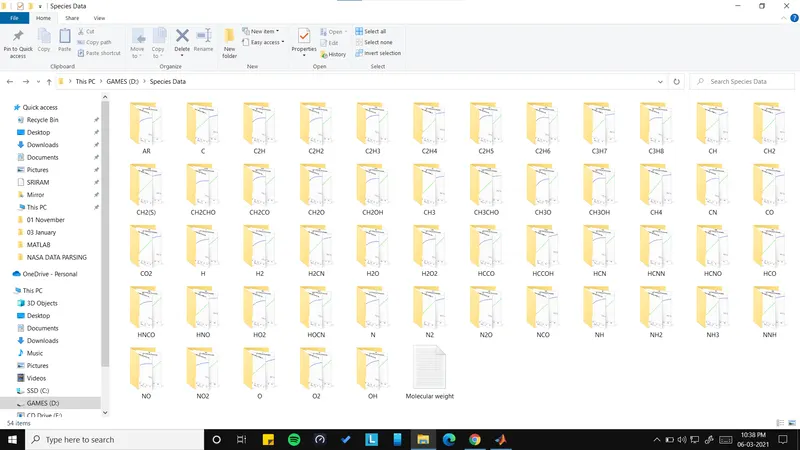
Intially, we are creating the main folder named "Species Data" into which sub-folders are created for the species. The reaosn to place this inside the forr loop is to name the sub-folders as per the species information segregated earlier.

CALCULATION:

For the calculation part, we need to work on the coefficients which are being concatenated and stored for each species. But the coefficients has to be separated and has to be converted from the character to numerical values for calculation. This is carried out as follows:

se = (strfind(jv{k},'E')); % searching the exponential in co-efficients

The se variable stores the exponential,E position in the concatenated line.

 % Creating local temperature range
    T = local_low_temp(k):local_high_temp(k);

Then we are creating temperature variable T, to store the local range of each species.

SPECIFIC HEAT:

   for t = 1:length(T)
        if T(t) >= min(local_low_temp(k)) || T(t) <= min(local_mid_temp(k))
            
s = 1; % index variable for exponential position
            
% specific heat for low to medium temperature local range
            cp{k}(t) = R.*(str2num(jv{k}(1:se(s)+3)) + str2num(jv{k}(se(s)+4:se(s+1)+3)).*T(t) + str2num(jv{k}(se(s+1)+4:se(s+2)+3)).*T(t)^2 + str2num(jv{k}(se(s+2)+4:se(s+3)+3)).*T(t)^3 + str2num(jv{k}(se(s+3)+4:se(s+4)+3)).*T(t).^4);

% specific heat for medium to high temperature local range
            cp{k}(t) = R*(str2num(jv{k}(1:se(s)+3)) + str2num(jv{k}(se(s)+4:se(s+1)+3)).*T(t) + str2num(jv{k}(se(s+1)+4:se(s+2)+3)).*T(t)^2 + str2num(jv{k}(se(s+2)+4:se(s+3)+3)).*T(t)^3 + str2num(jv{k}(se(s+3)+4:se(s+4)+3)).*T(t)^4);

The counter variable t is initiated from 1 to the length of the T, which is the value from the low temperature to the high temperature for the species.Then there is a if condition that checks whether the temperature at the current iteration is within the local to mid range then proceeds the calculation of the specific heat. In the mathematical part, we are separating the values with the exponential position determined earlier. And then converting them to the numerical values from character.

Among the 14 co-efficients, the first 7 are for the lower range and the rest for the higher range, the calculation is carried out for the same. The same above steps are repeated for enthalpy and entropy calculation with the corresponding changes in their formula.

ENTHALPY:

% Enthalpy heat for low to medium temperature local range
            H{k}(t) = R.*T(t).*( (str2num(jv{k}(1:se(s)+3))) + str2num(jv{k}(se(s)+4:se(s+1)+3)).*T(t)./2 + (str2num(jv{k}(se(s+1)+4:se(s+2)+3)).*(T(t)^2)./3) + (str2num(jv{k}(se(s+2)+4:se(s+3)+3)).*(T(t).^3)./4) + (str2num(jv{k}(se(s+3)+4:se(s+4)+3)).*(T(t).^4)./5) + (str2num(jv{k}(se(s+4)-10:se(s+4)+3))./T(t)));

% Enthalpy for medium to high temperature local range
            H{k}(t) = R.*T(t).*( (str2num(jv{k}(1:se(s)+3))) + str2num(jv{k}(se(s)+4:se(s+1)+3)).*T(t)./2 + (str2num(jv{k}(se(s+1)+4:se(s+2)+3)).*(T(t)^2)./3) + (str2num(jv{k}(se(s+2)+4:se(s+3)+3)).*(T(t).^3)./4) + (str2num(jv{k}(se(s+3)+4:se(s+4)+3)).*(T(t).^4)./5) + (str2num(jv{k}(se(s+4)-10:se(s+4)+3))./T(t)));

ENTROPY:

% Entropy for low to medium temperature local range
            S{k}(t) = R*((str2num(jv{k}(1:se(s)+3)).*log(T(t))) + str2num(jv{k}(se(s)+4:se(s+1)+3)).*T(t) + str2num(jv{k}(se(s+1)+4:se(s+2)+3)).*T(t)^2 + str2num(jv{k}(se(s+2)+4:se(s+3)+3)).*T(t)^3 + str2num(jv{k}(se(s+3)+4:se(s+4)+3)).*T(t)^4 + str2num(jv{k}(se(s+5)+4:se(s+6)+3)));

% Entropy for medium to high temperature local range
            S{k}(t) = R*((str2num(jv{k}(1:se(s)+3)).*log(T(t))) + str2num(jv{k}(se(s)+4:se(s+1)+3)).*T(t) + str2num(jv{k}(se(s+1)+4:se(s+2)+3)).*T(t)^2 + str2num(jv{k}(se(s+2)+4:se(s+3)+3)).*T(t)^3 + str2num(jv{k}(se(s+3)+4:se(s+4)+3)).*T(t)^4 + str2num(jv{k}(se(s+5)+4:se(s+6)+3)));

PLOTTING AND SAVING:

The calculated data now as to be plotted and saved.

At first we are determing the folders created for the species names.

% assigning sub folders respective to the species name
    mtd = fullfile('D:\','Species Data',sprintf(species_names{k}));
    cd(mtd); % making the same above as current directory to save graphs

The cd makes the current directory that is being created in the above line. The sprintf command returns the actual value of the species names as character.

Cp vs T:

% Cp vs T
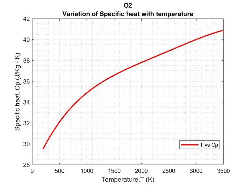
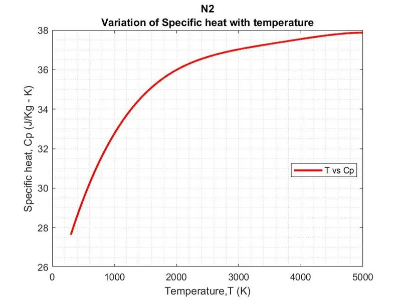
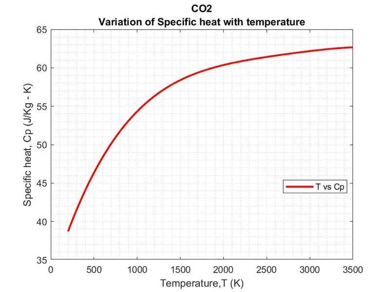
    plot_cp = plot(T(1:t),cp{k}(1:t),'linewidth',2,'color','r');

As usual, we are plotting the points of specific heat against the temperature using the plot command and specifying the width of the graph and color.

 % graph detailing
    title({sprintf(species_names{k}),'Variation of Specific heat with temperature'});
    legend('T vs Cp','location','best');
    xlabel('Temperature,T (K)');
    ylabel('Specific heat, Cp (J/Kg - K)');
    grid minor

Then appropriate detailing is made for the graph.

 saving plotted graphs to the respective species folder.
    saveas(gcf,'Specific_heat_vs_Temperature','jpeg');

We are using saveas feature to save the plotted graph. The gcf command gets the current figure, i.e the plotted graph of the current species and then saves it with the specified file name and extension.

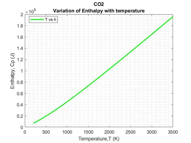
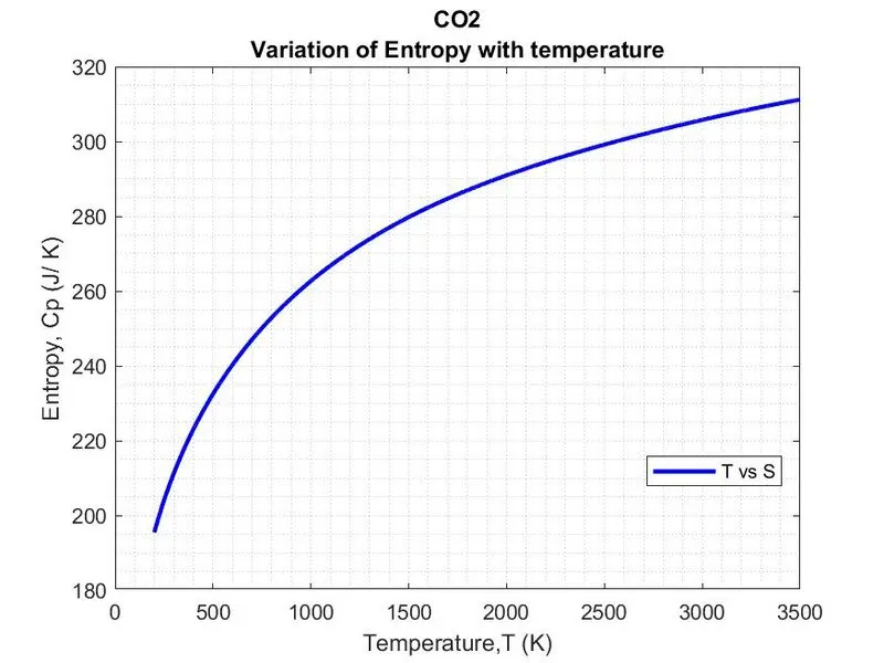
The same being repeated for enthalpy and entropy.

h vs T

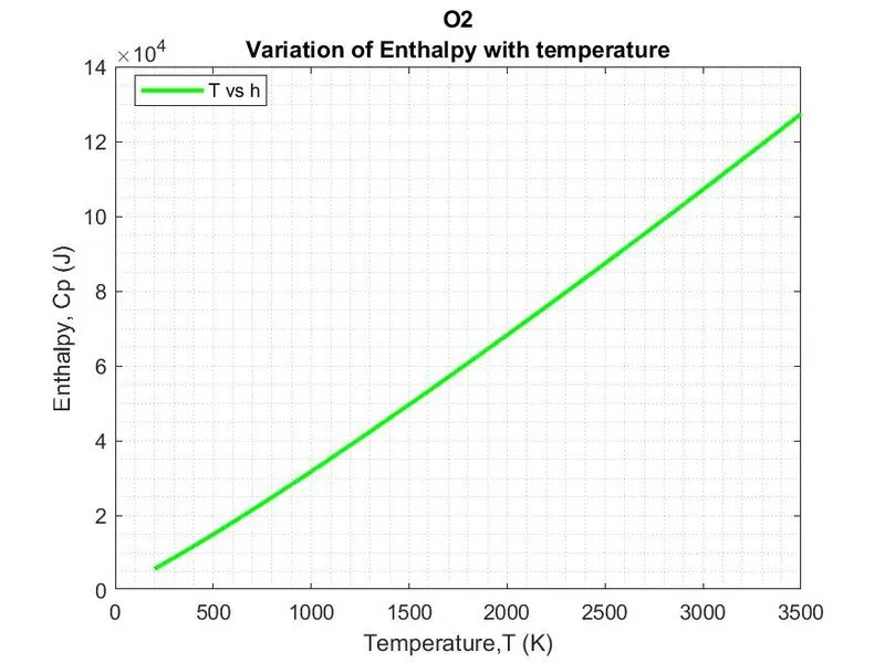
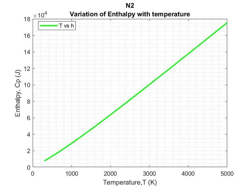
plot_H = plot(T(1:t),H{k}(1:t),'linewidth',2,'color','g');
    title({sprintf(species_names{k}),'Variation of Enthalpy with temperature'});
    legend('T vs h','location','best');
    xlabel('Temperature,T (K)');
    ylabel('Enthalpy, Cp (J)');
    grid minor
    saveas(gcf,'Enthalpy_vs_Temperature','jpeg');

S vs T

  
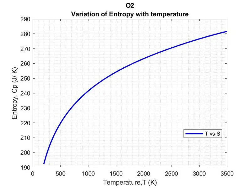
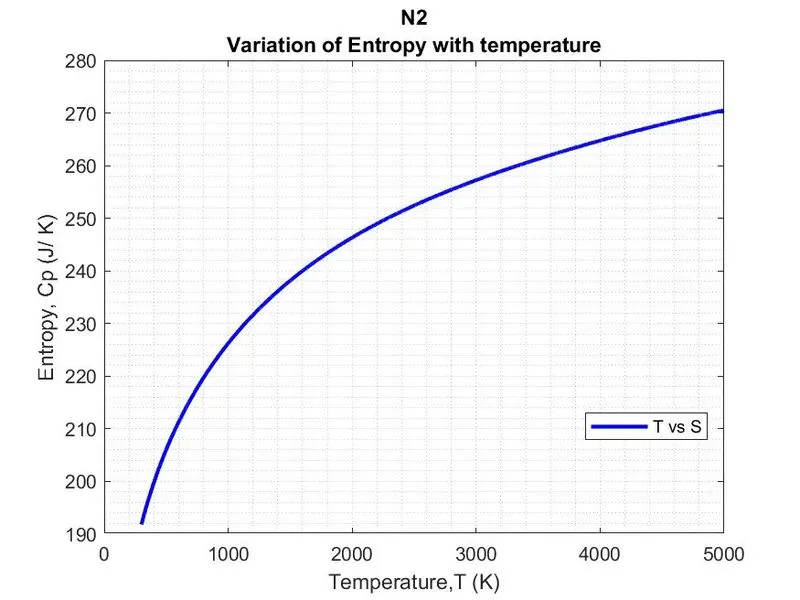
    plot_S = plot(T(1:t),S{k}(1:t),'linewidth',2,'color','b');
    title({sprintf(species_names{k}),'Variation of Entropy with temperature'});
    legend('T vs S','location','best');
    xlabel('Temperature,T (K)');
    ylabel('Entropy, Cp (J/ K)');
    grid minor
    saveas(gcf,'Entropy_vs_Temperature','jpeg');

MOLECULAR WEIGHT:

Initially, the molecules are initiated to the names variable and their respective atmoic weights are to the at_wt variable.

Then the molecular weight are initialized to 0.

% molecular weigh by chemical formula

% elements in the data file
names = {'O','H','C','N','AR'} ;
    
% valuing with their atomic weight
at_wt = [15.999, 1.00784, 12.011, 14.007, 39.948];

m_w = 0; % initial value for molecular weight variable

Now, the molecular weight of each compound has to be calculated as follows.

 % separating the species chemical formula
    n2c{k} = num2cell(species_names{k});

The num2cell function separates the cell array variables the into each single character. This is being used because the compound's chemical formula.

for t = 1:length(names)
        for inc3 = 1:length(species_names{k})
            if strcmp(n2c{k}(inc3),names(t)) == 1
                m_w = m_w + at_wt(t); % molecular weight for single molecule
                
            end
        end

The main for loop iterates till the length of the names variable. Then there is a nested for loop that iterates till the length of the species name. Then the string compare function is used to compare the components of the n2c variable and the names, where the variables are initiated corresponding to the chemical compounds in the species data.

Then the atomic weight of the respective compared variable is calculated.

Now, some compounds have molecules that has value more than one. For this there is another for loop created to calculate them as follows:

   % calculation for above 2 molecules of a compound
    for inc3 = 1:length(species_names{k})
        % determines whether the cell array value is a number  and
        % converts to number in array form from cell array character
        con_val = str2num(species_names{k}(inc3));
        
        if isempty(con_val)
            
            continue  % the iteration moves up if above condition satisfies
        else
            pos2 = inc3;
            num_val = str2double(species_names{k}(pos2));
            m_w = m_w + at_wt(pos2-1)*(num_val-1); % final molecular weight
            
        end
        
    end

The values are now determined whether they are numerical or not. For this we are converting the characters in the chemical formula to number. If there is a character, then the variable con_val is emptied. This is checked again in the isempty function.

If the value is a logical 1, then the iteration moves to the next incremented value. If it is a logical 0, then it proceeds the calculation.

Then we are calculating the moleculare weight again since there are more than one molecules in the compound. There is subtraction of unity

i) Since the same molecule is calculated earlier in the for loop

ii) In the position since the molecule count is for the precedent variable.

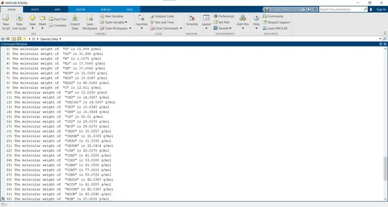
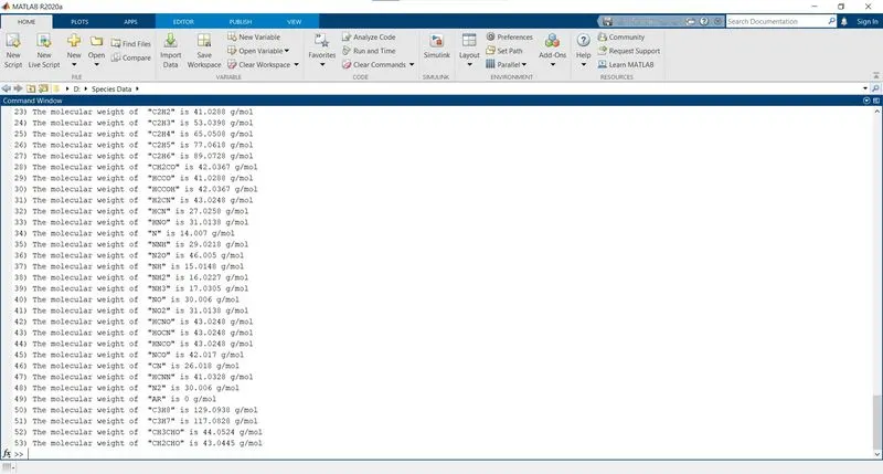
Finally, we are displaying the calculated molecular weight as follows:

% Output display
    output_disp = [num2str(k),')' ' The molecular weight of  ','"', sprintf(species_names{k}),'"',' is ',num2str(m_w),' g/mol.n'];
    disp(output_disp);

Also, we are storing the above calculated data and display to a text file that contains all the species molecular weights.

We are opening the file with a reference variable fid2, Then we are specifying the file name, extension and the operation we are going to carry out in the file. Writing into the file, hence the expression 'w'.

Then fprintf to write the data. The pointer reference variable and the display output variable. Then the new line command to format the data.

fid2 = fopen('Molecular weight.txt','w');
fprintf(fid2,output_disp); % writing in the opened text file
    fprintf(fid2,'\n');
fclose(fid2); % closing the file

USER BASED INPUT:

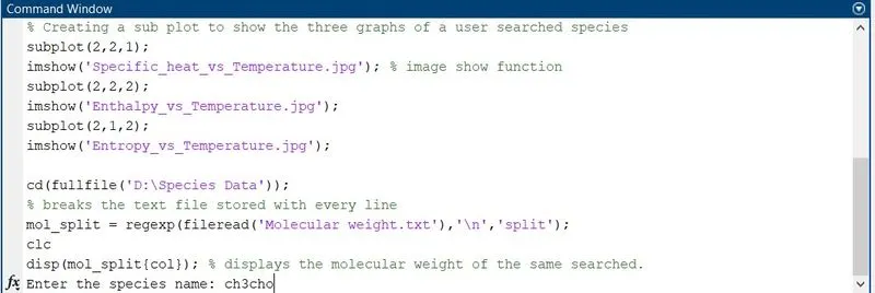
The x variable stores the chemical compound of the species from the user, and the 's' returns the entered text, without evaluating the input as an expression.

Then the strcmpi makes a case insensitive comparison of the input with the species data available. The col variable stores the index of the found species.

% user input based
x = input('Enter the species name: ','s'); % input from the user

for k = 1:length(jv)
    % compares the input value with the species data
    if strcmpi(species_names_cell{k}(1),sprintf((x))) == 1
        col = k; % gives the indices value of the above searched.
    end
end

GRAPH DISPLAY:

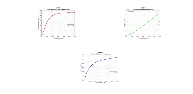
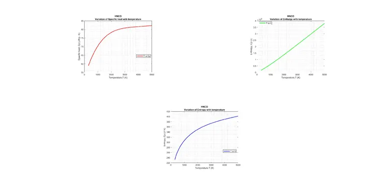
Then we are displaying the corresponding graphs of the species by using subplot commands.

% Creating a sub plot to show the three graphs of a user searched species
subplot(2,2,1);
imshow('Specific_heat_vs_Temperature.jpg'); % image show function
subplot(2,2,2);
imshow('Enthalpy_vs_Temperature.jpg');
subplot(2,1,2);
imshow('Entropy_vs_Temperature.jpg');

MOLECULAR WEIGH:

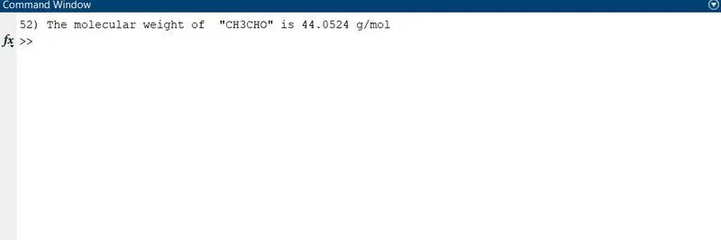
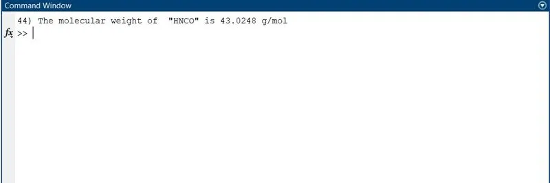
Then we are accessing the text file created and then displaying the molecular weight of the species. Again we are using the regular expression method and then displaying the output by comparing species number against the number line of the text file.

% breaks the text file stored with every line
mol_split = regexp(fileread('Molecular weight.txt'),'\n','split');
clc
disp(mol_split{col}); % displays the molecular weight of the same searched.

OUTPUT:

The output folder created and the sub-folders.

PLOTTED GRAPHS:

The graphs obtained for the respective species are as follows:

O2:

N2:

CO2:

MOLECULAR WEIGHT:

USER BASED OUTPUT:

The user based input search for the species output is as follows:

CH3CHO:

HNCO: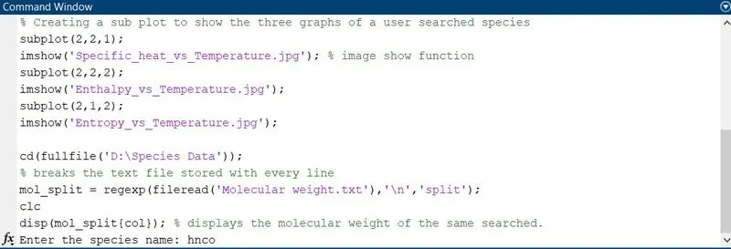

REFERENCES:

MATLAB community forum