Week 4 - Genetic Algorithm

AIM: To write a code in MATLAB to optimise the stalagmite function and find the global maxima of the function.

OBJECTIVES:

• To explain the concept of genetic algorithm
• To write a code in MATLAB to optimise the stalagmite function and find the global maxima of the function.
• To plot graphs for all 3 studies and for F maximum vs no. of iterations

INTRODUCTION

Optimization deals with problems of minimizing or maximizing a function with several variables usually subjected to equality and/or inequality constraints. It plays central role in operations research, management science and engineering design. Many engineering design problems are very complex and difficult to solve using conventional optimization technique. In recent years Genetic Algorithms have received considerable attention regarding their potential as a novel optimization technique.

GENETIC ALGORITHM

Theory about Genetic Algorithm

Genetic Algorithm is a search based optimization technique based on the principles of genetics and natural selection. It is used to find the optimal or near optimal solutions to complex engineering problems. Genetic Algorithms are a subset of a much larger branch of computation known as Evolutionary Computation.

GAs were developed by John Holland and his colleagues at University of Michigan. In GAs we have a pool or population of possible solutions to the given problem. These solutions will then undergo recombination and mutation, producing new children and the process is repeated over various generations. Each individual is assigned a fitness value and the fitter individuals are given a higher chance to mate and yield more fitter individual. This is in line with the Darwinian Theory of Survival of Fittest.

Basic Terminology

1. Population: It is a subset of all the possible solutions to the given problem
2. Chromosomes: A chromosome is one such solution to the given problem
3. Gene: a gene is one element position of the chromosome
4. Allele: It is the value of a gene takes for a particular chromosome.
5. Genotype: Genotype is the population in the computation space
6. Phenotype: It is the population in the actual real world solution space.
7. Decoding: It is a process of transforming a solution from the genotype to the phenotype space.
8. Encoding: It is a process of transforming from the phenotype to genotype space.

Basic structure

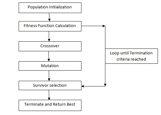
The basic structure of GAs is as follows –

We start with initial population, select parents from this population for mating. Apply crossover and mutation operators on the parents to generate the new off-springs. And finally these off-springs replace the existing individuals in the population and the process repeats.In this way GAs actually try to mimic the human evolution to some extent.

GAs Termination Condition

The termination condition of a GA is important in determining when a GA run will end. It has been observed that initially, the GA progresses very fast with better solutions coming in every few iterations. But this tends to saturate in the later stages where the improvements are very small. We usually want a termination condition such that our solution is very close to the optimal, at the end of the run.

Usually we keep the one of the following termination conditions –

• When there has been no improvement in the population for X iterations
• When we reach an absolute number of generations
• When the objective function value has reached a certain pre-defined value.

Syntax for GA

There are several ways to define the GA function depending on the problem being solved. The syntax used for this study is shown below

• x = ga(fun,nvars)

Where, x = optimal solution

fun = Objective function

nvars = Number of variables

• x = ga(fun,nvars,A,B,Aeq,Beq,lb,ub)

Where, A,B = Linear inequality constraints

Aeq, Beq = Linear equality constraints

If there are no linear inequality and equality constraints, then A,B,Aeq,Beq are set to [ ]

• x = ga(fun,nvars,A,B,Aeq,Beq,lb,ub,nonlcon,IntCon,Options)

Where, nonlcon = Nonlinear constraints

IntCon = Integer values

Options = Optimization options

If there are no nonlinear constraints and integer values then nonlcon and Intcon are set to [ ]

Stalagmite Function

The stalagmite function is defined below:

`f(x,y)= f_(1,x) f_(2,x) f_(1,y) f_(2,y)`

Where,

`f_(1,x)=[sin⁡(5.1πx+0.5)]^6`

`f_(1,y)=[sin⁡(5.1πy+0.5)]^6`

`f_(2,x)=exp⁡[-4ln⁡(2) (x-0.0667)^2/0.64]`

`f_(2,y)=exp⁡[-4ln⁡(2) (y-0.0667)^2/0.64]`

MATLAB CODE

1. Stalagmite Function code

%for calling stalagmite function
function[f]=stalagmite_funct(input)
x=input(1)
y=input(2)
f1_x=(sin(5.1*pi*x+0.5)).^6;
f1_y=(sin(5.1*pi*y+0.5)).^6;
f2_x=exp(-4*(log(2)))*((x-0.0667).^2)/0.64;
f2_y=exp(-4*(log(2)))*((y-0.0667).^2)/0.64;
f=-(f1_x*f1_y*f2_x*f2_y) %negative sign for finding global maximum

2. Code to get stalagmite function

function[f]=get_stalagmite(xx,yy)
for i=1:length(xx)
    for j=1:length(yy)
    input_vector(1)=xx(i,j);
    input_vector(2)=yy(i,j);
    f(i,j)=stalagmite_function(input_vector);
    end
end
end

3.Code to evaluate maxima of the function

close all
clear all
clc
 
%defining search space
x=linspace(0,0.6,150);
y=linspace(0,0.6,150);
 
%converting into two dimensional array
[xx,yy]=meshgrid(x,y);
num_iterations=50
f=get_stalagmite_fun(xx,yy);

tic
%case 1
for i=1:num_iterations
    [inputs,fopt(i)]=ga(@stalagmite_function,2);
    xopt(i)=inputs(1);
    yopt(i)=inputs(2);
end
case1_time=toc
figure(1)
subplot(2,1,1)
hold on
surfc(xx,yy,-f)
shading interp
plot3(xopt,yopt,-fopt,'marker','o','markersize',5,'markerfacecolor','r')
title('Unbounded Inputs')
subplot(2,1,2)
plot(fopt)
xlabel('Number of Iterations')
ylabel('Function Maximum')
 
%case2 - with upper and lower bounds
tic
for i=1:num_iterations
    [inputs,fopt(i)]=ga(@stalagmite_function,2,[],[],[],[],[0;0],[0.6;0.6]);
    xopt(i)=inputs(1);
    yopt(i)=inputs(2);
end
case2_time=toc;
figure(2)
subplot(2,1,1)
hold on
surfc(xx,yy,-f)
shading interp
plot3(xopt,yopt,-fopt,'marker','o','markersize',5,'markerfacecolor','r')
title('Bounded Inputs')
subplot(2,1,2)
plot(fopt)
xlabel('Number of Iterations')
ylabel('Function Maximum')
 
%case 3-increasing ga iterations
options=optimoptions('ga')
options=optimoptions(options,'populationSize',170);
tic
for i=1:num_iterations
    [inputs,fopt(i)]=ga(@stalagmite_function,2,[],[],[],[],[0;0],[0.6;0.6]);
    xopt(i)=inputs(1);
    yopt(i)=inputs(2);
end
case3_time=toc;
figure(3)
subplot(2,1,1)
hold on
surfc(xx,yy,-f)
shading interp
plot3(xopt,yopt,-fopt,'marker','o','markersize',5,'markerfacecolor','r')
title('Bounded Inputs')
subplot(2,1,2)
plot(fopt)
xlabel('Number of Iterations')
ylabel('Function Maximum')

CODE EXPLANATION

1. Linspace command stores 150 values of x from 0 to 0.6 and 150 values of y from 0 to 0.6. Meshgrid command is used to create a 2D array using the arrays x and y.
2. For assigning values to variables input(1) and input(2), two for loops are used. Calling the function stalagmite that contains the code evaluates the value of function.
3. In Case 1, an attempt is made to reach global maximum without knowing the search space. In other words upper and lower bounds are not defined. So chances of getting optimum solution is minimum
4. In Case2, attempt is made reach the global maximum by defining upper and lower bounds i.e. between 0 to 0.6. In this case chances of getting global maximum is improved.
5. In case3, attempt is made to reach global maximum by increasing number of GA iterations and accuracy is improved than the previous cases

ERRORS

Action taken: Parameter name 'population size' was replaced by 'populationSize'.

OUTPUT

Case1: Statistical behavior with unbound inputs

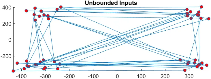
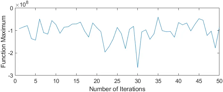
Observation: In Case 1, an attempt is made to reach global maximum without knowing the search space. In other words upper and lower bounds are not defined. So chances of getting optimum solution is minimum.

Case 2: Statistical behavior with bounded inputs

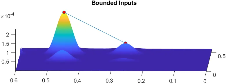
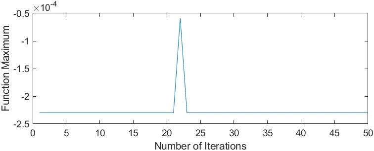
Observation: In Case2, attempt is made reach the global maximum by defining upper and lower bounds i.e. between 0 to 0.6. In this case chances of getting global maximum is improved except few iterations.

Case3:

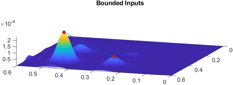
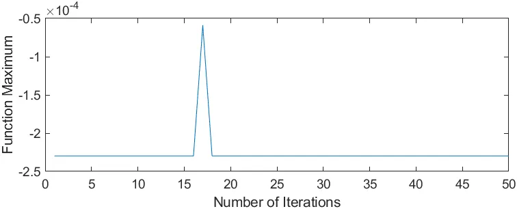
Observation: In case3, attempt is made to reach global maximum by increasing number of GA iterations and accuracy is improved than the previous cases. Result is found to be approximately 2.4*10^-4

REFERENCES

https://www.tutorialspoint.com/genetic_algorithms/genetic_algorithms_quick_guide.htm