Week 3 - Solving second order ODEs

AIM

To write a program in MATLAB that will simulate the pendulum motion

OBJECTIVES

• Reduction of 2^nd order ODE to 1^st order ODE
• To write the MATLAB program to solve ODE
• Stepwise explanation of the code
• Writing a note on errors fixed while programming
• Generation of animation

GOVERNING EQUATIONS

A simple pendulum is one which can be considered to be a point mass suspended from a string or rod of negligible mass. The equation that describes the motion of the pendulum is as follows

`(d^2 θ)/(dt^2 )+ (b/m) dθ/dt+(g/l)sinθ=0`

Where,

g = Acceleration due to gravity,

l = Length of the pendulum,

m = Mass of the pendulum,

b = Damping coefficient

Given input values are,

g = 9.81

l = 1

m = 1

b = 0.05

In MATLAB solution for first order ODE’s can be calculated using the inbuilt function ‘ode45’. Hence given second order ODE must be reduced to two first order ODE’s.

Let `θ= θ1`

The equation becomes,

`(d^2 θ1)/(dt^2 )+ (b/m) dθ1/dt+(g/l)sinθ1=0`

Also assume `dθ1/dt= θ2`

Then above equation can be rewritten as

`dθ2/dt+ (b/m)θ2+(g/l)sinθ1=0`

From the above two equations,

`dθ1/dt= θ2`----------------------------------------------------(1)

`dθ2/dt = - (b/m)θ2-(g/l)sinθ1`---------------------------------(2)

By these two equations we get values of `θ1 and θ2`

MATLAB CODE

clear all
close all
clc
 
%inputs
b=0.05 %damping coefficient
g=9.81 %acceleration due to gravity
l=1 %length of the pendulum
m=1 %mass of the pendulum
 
%initial conditions
theta_0=[0;3]; %initial displacement and initial velocity
 
%time points
t_span=linspace(0,10,500)
 
%solve ODE
[t results]=ode45(@(t,theta)odefun(t,theta,b,g,l,m),t_span,theta_0)
 
%plotting
plot(t,results(:,1)) 
hold on
plot(t,results(:,2))
ylabel('Plot')
xlabel('Time')
%animation of pendulum
ct=1
theta=results(:,1)
for i=1:length(theta)
    theta1=theta(i);
    x0=0
    y0=0
    x1=l*sin(theta1);
    y1=-l*cos(theta1);
    figure(1)
    plot([-1 1],[0 0],'linewidth',5,'color','b');
    hold on
    plot([x0 x1],[y0 y1],'linewidth',5,'color','g');
    hold on
    plot(x0,y0,'H','markersize',10,'MarkerEdgeColor','g','MarkerFaceColor','r');
    plot(x1,y1,'O','markersize',30,'MarkerEdgeColor','r','MarkerFaceColor','g');
    axis([-1.5 1.5 -1.5 0.5])
    pause(0.03)
    hold off
    M(ct)=getframe(gcf)
    ct=ct+1
end
 
%making the animation
movie(M)
videofile=VideoWriter('pendulum1.avi','uncompressed AVI')
open(videofile)
writeVideo(videofile,M)
close

MATLAB CODE FOR ode45 FUNCTION

function[dtheta_dt]=odefun(t,theta,b,g,l,m)
theta1=theta(1);
theta2=theta(2);
dtheta1_dt=theta2;
dtheta2_dt=-(b/m)*theta2-(g/l)*sin(theta1);
dtheta_dt=[dtheta1_dt;dtheta2_dt];
end

CODE EXPLANATION

Coding involves following steps

• First step is defining all the input values in the program
• Second step is calling ode45 function.Ode45 is a function in matlab that solves ordinary or partial differential equations using a numerical method. In a separate MATLAB code ode solver is defined.
• Final step is plotting the results and generation of animation. Animation is generated by constructing a for loop.

ERRORS

Error in calling ode45 function

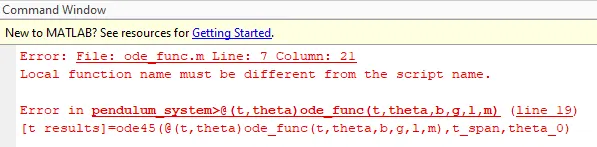
Error fixed by changing the calling function syntax

[t results]=ode45(@(t,theta)odefun(t,theta,b,g,l,m),t_span,theta_0)

(ode_func is replaced by odefun)

OUTPUT

1. Angular velocity and Angular displacement plot is shown below

x-axis: Time

y-axis: Angular velocity (Red color) and Angular displacement (Blue color)

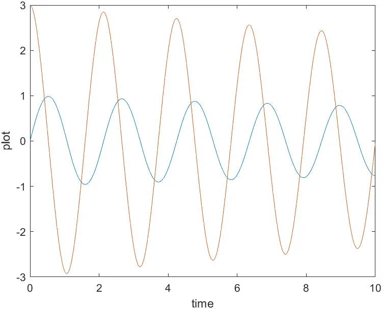
Observation: Both Angular velocity and Angular displacement is decreasing at very slow rate. In other words it is very slow damping process

2. Animation is uploaded to youtube whose link is provided below

https://youtu.be/Rs0fnCRJouo