Optimize the Stalagmite function using Genetic Algorithm in MATLAB.

Aim: Write a code to optimize the stalagmite function using MATLAB

Objective:

• Write a code for the stalagmite function using “ga(genetic algorithm)” command.
• Find the global maxima for the function.
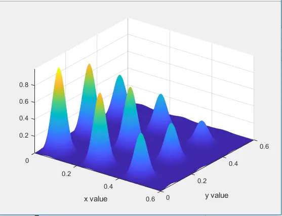
• Plot stalagmite function and 3 studies showing the global maxima.

Theory:

General Algorithm(GA/ga):

A Genetic Algorithm is a method to optimize a given objective function that is either constrained or non-constrained that is based on natural selection, the process that drives biological evolution. The genetic algorithm repeatedly modifies a population of individual solutions. At each step, the genetic algorithm selects individual at random from current population to be parents and use them to produce the children for next generation. Over a successive generation, the population “evolves” towards an optimal solution.

The genetic algorithm applies three main rules at each step to create next-generation from a given population,

• Selection: select the individual for creating children for the next generation.
• Cross-Over: Mate two-parent to form children for next generation.
• Mutation: make random changes to parents to form a child

Syntax use for genetic algorithm:

x = ga(fun,nvras)

x = ga(fun,nvras,A,b,Aeq,beq,lb,ub)

x = ga(fun,nvras,A,b,Aeq,beq,lb,ub,nonlcon,IntCon,options)

Where,

ga = genetic algorithm

fun = function

nvras = number of independent variable

A,b = linear inequality function

Aeq = matrix for linear equality constrained

Beq = vector for linear equality constrained

lb = lower bound

ub = upper bound

nonlcon = non linear constrained

Intcon = integer constrained

options = options created by using optimoptions

Given Equation:

Global minima find by

f = f₁*f₂*f₃*f₄

Global maxima is find by

f = -( f₁*f₂*f₃*f₄₎

Where,

f₁ = [sin(5.1x+0.5)]⁶

f₂ = [sin(5.1y+0.5)]⁶

f₃ = exp[-4log(2)*((x-0.0667)^2/0.64)]

f₃ = exp[-4log(2)*((y-0.0667)^2/0.64)]

Commands:

• Linspace
• Meshgrid
• For loop
• Surfc
• Shading interp

CODE:

MAIN CODE:

clear all
close all
clc

% input array of x and y
x = linspace(0,0.6,150);
y = linspace(0,0.6,150);

% creating a 2 dimensional array
[xx,yy] = meshgrid(x, y);

% evaluating the stalagemaite function
for i = 1:length(xx)
    for j = 1:length(yy)
        input_vector(1) = xx(i,j);
        input_vector(2) = yy(i,j);
        f(i,j) = stalagmite(input_vector);
    end
end
 

surfc(xx,yy,-f)
xlabel('x value');
ylabel('y value');
shading interp

[inputs, fval] = ga(@stalagmite,2)   % genetic algorithm

Explanation:

• Start the code using the command clear all, close all, and clc for clear, close, cancel previous data store in the workspace, command, and editor window.
• Then by using linspace command to create an equally spaced one-dimensional array for x, and y variables.
• To convert one dimensional into 2D use “meshgrid” command, which is used to evaluate of function of two variables and the 3D surface plot.
• To do iteration for population use “for loop” giving proper inputs.
• Then call the “stalagmite” function to create stalagmite for a given equation.
• Use “surfc” to display data which is a function of two variables,to hide grid shows on stalagmite use “shading interp”.
• To show ‘final value’ and ‘inputs use “ga” command. Syntax of “ga” for this problem is’

ga(@stalagmite,2)
PLOT:

FUNCTION CODE:

stalagmite function

function[f]=stalagmite(input_vector)

x = input_vector(1);
y = input_vector(2);
f1 = (sin(5.1*pi*x+0.5))^6;
f2 = (sin(5.1*pi*y+0.5))^6;
f3 = exp(-4*log(2)*((x-0.0667)^2/0.64));
f4 = exp(-4*log(2)*((y-0.0667)^2/0.64));

f=-(f1.*f2.*f3.*f4);
end

Explanation:

• Function code is very similar to script file but with some certain differences, basically, it accepts input argument and returns output argument.
• Define the function in MATLAB. Always remember that the main code and function code is in the same folder.
• The genetic algorithm always finds minima, to find maxima put negative “-” sign to a given function.
• So observation says , after running the “ga” the final value changes every time. So for reach to one optimal solution, we go through some studies.

CODE:

clear all 
close all
clc

% defining our search space
x = linspace(0,0.6,150);
y = linspace(0,0.6,150);
num_cases = 50;

% create 2D array
[xx, yy] = meshgrid(x,y);
 
% evaluating the stalagmite function

for i = 1:length(xx)
    for j = 1:length(yy)
        input_vector(1) = xx(i,j);
        input_vector(2) = yy(i,j);
        f(i,j) = stalagmite(input_vector);
    end
end

tic
%study 1- statastical behaviour
for k = 1:num_cases;
    [inputs,fopt(k)] = ga(@stalagmite,2);
    xopt(k) = inputs(1);
    yopt(k) = inputs(2);
    
end
study1_time = toc

figure(1)

subplot(2,1,1)
surfc(xx,yy,-f);
shading interp
hold on
plot3(xopt,yopt,-fopt,'marker','o','markersize',3,'markerfacecolor','r')
title('unbounded inputs')
subplot(2,1,2)
plot(fopt)
xlabel('Iteration')
ylabel('function minimum')



tic
%study 2- statastical behaviour with upper and lower bound
for k = 1:num_cases;
    [inputs,fopt(k)] = ga(@stalagmite,2,[],[],[],[],[0;0],[0.3;0.3]);
    xopt(k) = inputs(1);
    yopt(k) = inputs(2);
    
end
study2_time = toc

figure(2)

subplot(2,1,1)
surfc(xx,yy,-f);
shading interp
hold on
plot3(xopt,yopt,-fopt,'marker','o','markersize',3,'markerfacecolor','r')
title('bounded inputs')
subplot(2,1,2)
plot(fopt)
xlabel('Iteration')
ylabel('function minimum')


tic
%study 3 increasing GA iteration
options = optimoptions('ga');
options = optimoptions(options,'populationsize',100)
for k = 1:num_cases;
    [inputs,fopt(k)] = ga(@stalagmite,2,[],[],[],[],[0;0],[0.3;0.3],[],[],options);
    xopt(k) = inputs(1);
    yopt(k) = inputs(2);
    
end
study3_time = toc
figure(3)

subplot(2,1,1)
surfc(xx,yy,-f);
shading interp
hold on
plot3(xopt,yopt,-fopt,'marker','o','markersize',3,'markerfacecolor','r')
title('bounded inputs')
subplot(2,1,2)
plot(fopt)
xlabel('Iteration')
ylabel('function minimum')

STUDY 1- STATISTICAL BEHAVIOUR

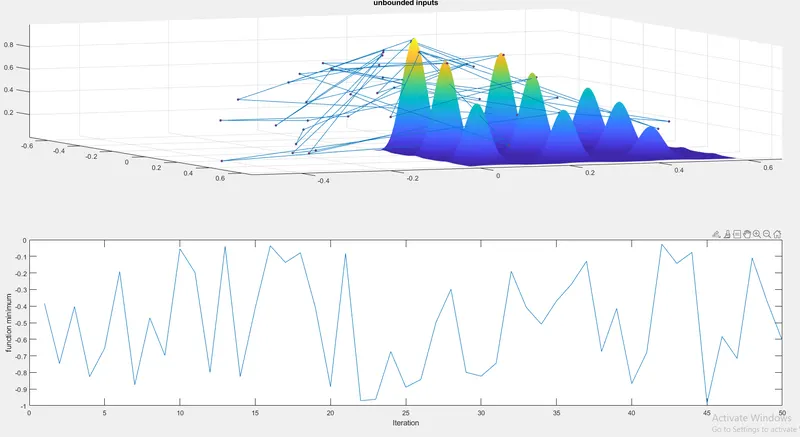
• In this study, we not providing bounds to “ga”, so it gives results beyond specified search space.
• Then use “for loop” to do iteration till num_cases.
• Then open a new figure window, using the “subplot” command to create a number of plots in the same figure window.
• Use “surfc”to display data which is a function of two variables, to hide grid shows on stalagmite use “shading interp”.
• Then use the “plot3” command to plot “xopt,yopt,fopt” over the 50 studies in one plot, it shows how the “ga” is performing.
• In the second subplot, we plot the “fopt” that function is predicted.
• With the help of the “tic & toc” command, we measure the time required for simulation.

PLOT:

STUDY 2- STATISTICAL STUDY WITH UPPER ABD LOWER BOUND

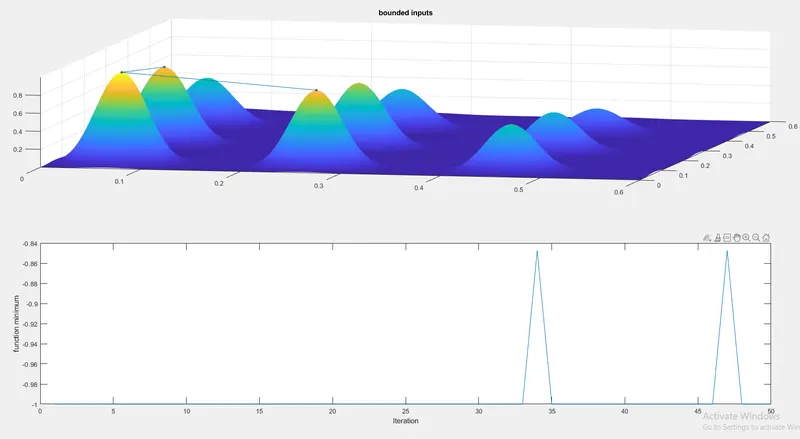
In this study, we provide upper and lower bound to “ga” for shows the result within search space gives to the independent variable.

“ga” Syntax used for this study is,

x = ga(fun,nvras,A,b,Aeq,beq,lb,ub)

PLOT:

STUDY 3- INCREASING “GA” ITERATION

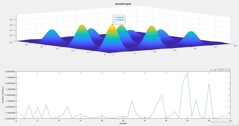
• I addition with upper and lower bound increase population size. We know “ga” works on random sampling method, So to increase the performance of “ga” increase population size, using command “optimoptions”.
• Also with less population size, we only find local minima or maxima, to find global maxima or minima we have to increase the population size
• Here is one disadvantage, increasing the size of the population increase the simulation time

PLOT:

Error:

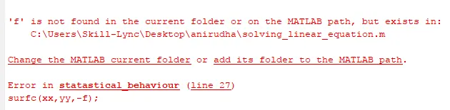
The following error shows because the value of "f" is not present in the current folder and also in the study code. To overcome this introduce function using for loop.

CONCLUSION:

In this way, we find the global maxima at (x=0.0668344,y=0.0668362,z=1)