OTTO CYCLE EFFICIENCY AND PLOT P-V DIAGRAM USING 'MATLAB'

• AIM: To write a program for the Otto cycle using MATLAB.
• OBJECTIVE:

• Create code for Otto cycle using MATLAB command and syntax.
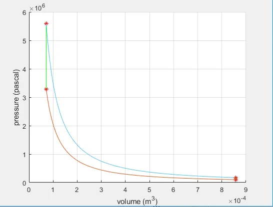
• Plot a P-V diagram to show different process occurs in the Otto cycle.
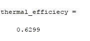
• Find the thermal efficiency of the engine.

• THEORY:

• Engine: A device that converts Thermal energy into Mechanical energy or Kinetic energy or any useful work.
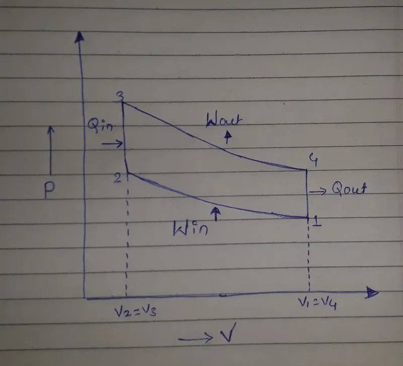
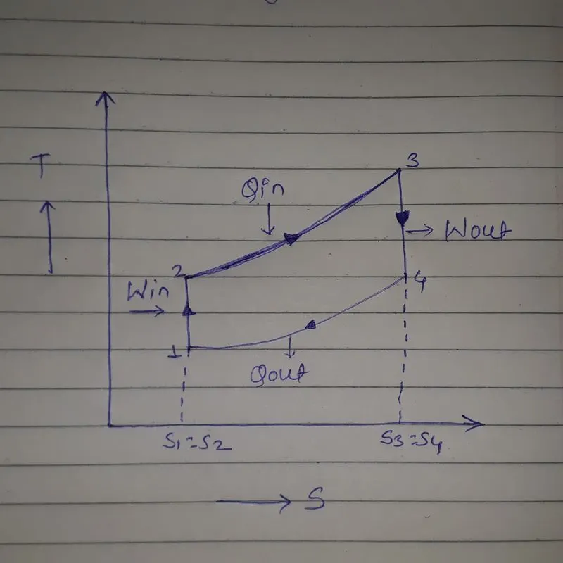
• Otto cycle: an otto cycle is an idealized thermodynamic cycle that describes the functioning of a typical spark ignition piston engine. the otto cycle is a description of what happens to the mass of gas as it is subject to changes of pressure, volume, temperature, the addition of heat, and removal of heat.

• P-V and T-S diagram:

• Equation :

• Change of volume inside the combustion chamber is given by

V = 1+(r_c-1)[R+1-cosθ-(R²-sin²θ)^1/2]

• Swept volume: the volume swept by the piston during its motion.

Vs = pi/4*d²*l

Where d = diameter of the bore ;

l = height of the piston

• Clearance volume: it is the volume between piston and top dead center during combustion and exhaust stroke.

Vc = [Vs/(rc-1)]

• Total volume: it is the addition of a swept volume of the cylinder and clearance volume

Vt = Vc+Vs

• Adiabatic process: is a type of thermodynamic process which occurs without transferring heat or mass between system and its surrounding.

PV^γ = C

Where, P = pressure,

V = volume,

C = constant

• Combined Gas law: It is stated that the ratio of the product of pressure and volume to its absolute temperature is equal to constant.

PV/T = C

Where, P = pressure,

V = volume,

T = temperature,

C = constant

• CODE:
• MAIN CODE:

 clear all
 close all
 clc
 % input
 gamma = 1.4;    
 t3 = 2300;        % in kelvin
 
 % state variable
 p1 = 101325;      % in pa
 t1 = 500;         % in kelvin
 
 % engine geomtric parameter
 bore = 0.1;          % in meter
 stroke = 0.1;        % in meter
 con_rod = 0.15;      % in meter
 cr = 12;
 
 % calculating the swept volume and the clearance volume
 v_swept = (pi/4)*bore^2*stroke;
 v_clearance = v_swept/(cr-1);
 
 v1 = v_swept+v_clearance;
 v2 = v_clearance;
 
 % state variable at state point 2
 % p2v2^gamma = p1v1^gamma
 % p2 = p1(v1/v2)^gamma = p1*cr^gamma
 p2 = p1*cr^gamma;
 
 % p1v1/t1 = p2v2/t2 then
 % t2 = p2v2t1/(p1*v1)
 t2 = p2*v2*t1/(p1*v1);
 
 % to create volume and pressure array
 constant_c =p1*v1^gamma;
 V_compression = engine_kinematics(bore,stroke,con_rod,cr,180,360);
 
 P_compression  = constant_c./V_compression.^gamma;
 
 % state variable at state point 3
 v3 = v2;
 
 % p3v3/t3 = p2v2/t2 then
 % p3 = p2*t3/t2
 p3 = p2*t3/t2;
 
 % to create volume and pressure array
 constant_c =p3*v3^gamma;
 V_expansion = engine_kinematics(bore,stroke,con_rod,cr,0,180);
 
 P_expansion  = constant_c./V_expansion.^gamma;
 
 % state variable at state point 4
 v4 = v1
 
 % p3v3^gamma = p4v4^gamma then
 % p4 = p3*(v3/v4)^gamma
 p4 = p3*(v3/v4)^gamma;
 
 % thermal efficiency
 thermal_efficiecy = 1-((cr)^(1-gamma))
 
 figure(1)
 hold on
 plot(v1,p1,'*','color','r')
 plot(V_compression,P_compression)
 plot(v2,p2,'*','color','r')
 plot([v2 v3],[p2 p3]','color','g')
 plot(v3,p3,'*','color','r')
 plot(V_expansion,P_expansion)
 plot(v4,p4,'*','color','r')
 plot([v1 v1],[p4 p1]','color','g')
 grid on
 xlabel('volume (m^3)')
 ylabel('pressure (pascal)')
 

• Procedure:

• Start program with a basic command for clear, close, cancel all previous data store in workspace and command window and also in the editor window, the command is as follows,

Clear all

Close all

Clc

• Then give the required inputs for the given code which are as follows

Gamma = 1.4,

Temperature(t3) = 2300 k,

• Introduce state variable for state1 which are as follows’

Pressure (p1) = 101325 Pa

Temperature (t1) = 500 k

• There are some engine geometric parameter so put that in the given code

Bore = 0.1 m

Stroke = 0.1 m

Connecting rod = 0.15 m

Compression ratio(cr) = 12

• Now, find the values of swept volume, clearance volume, and pressure and volume for corresponding states using the given formulas.
• Then to avoid more complexity in the program to trace the appropriate curve of constant volume in the P-V diagram, create a function say engine_kinematics. Then call this function to the main code. Keep always in mind that the function name and file name where the file will same is the same for call the function code in the main code.
• After these plot the P-V diagram using the ‘plot’ command and provide the required variable. give the ‘hold on’ command for the overlapping curve. To turn on the grid use the‘ grid on’ command.
• And finally, assign labels to the x and y-axis using the ‘label’ command.

• FUNCTION CODE:

function[V] = engine_kinematics(bore,stroke,con_rod,cr,start_crank,end_crank)

a = stroke/2;
R = con_rod/a;

v_s = pi/4*bore^2*stroke;      % swept volume
v_c = v_s/(cr-1);             % clearance volume

theta = linspace(start_crank,end_crank,100);

term1 = 0.5*(cr-1);
term2 = R+1-cosd(theta);
term3 = (R^2-sind(theta).^2).^0.5;

V = (1+term1*(term2-term3)).*v_c;

end

• A function in MATLAB is similar to Script files in MATLAB, but with certain differences. The function accepts the input argument and returns the output argument.
• Procedure:

• Assign the name here is engine_kinematics to the function, make sure the function name and film where the file is saved is the same.
• Give input to function as below

a = stroke/2

R = con_rod/a

• Then make an array of theta using the command ‘linspace’ of 100 values.
• Then assign the equation for ‘change of volume inside the combustion chamber is given by

V = [1+0.5*(cr-1)[R+1-cosd(theta)-(R^2-sind(theta).^2).^0.5]]*v_c;

• Then finish the program using the ‘end’ command.

• PLOT:

• RESULT:

Thermal efficiency = 0.6299

• CONCLUSION:

1. In this way, we plot the P-V diagram successfully.
2. The thermal efficiency of an engine is calculated as 0.6299.