CURVE FITTING using MATLAB
Aim: Write a code to curve fitting using MATLAB.
Objective:
- Write a code to fit a linear and cubic polynomial for Cp data.
- Write a code to a cubic polynomial using split.
- Plot the linear and cubic fit curve along with the data point.
Theory:
Curve fitting:
- Curve fitting is the process of constructing a curve or mathematical function, that has the best fit to a series of data points, possibly subject to constraints.
- Curve fitting can involve either interpolation, where an exact fit to the data is required, or smoothing, in which a "smooth" function is constructed that approximately fits the data.
Curve fitting function:
- The first-degree polynomial equation.
y = ax+b
- The third degree or cubic polynomial equation.
y = ax3+bx2+cx+d
Parameter:
There are some parameters to measure the goodness of the curve fit, which are as follows,
- Sum of square due to error(SSE)
- R-Square
- Adjusted R-Square
- Root Mean Square Error(RMSE)
Sum of square due to error(SSE):
This measures the total deviation of the response values from the fit to the response values.
A value close to ‘0’ shows the better fit
SSE = 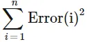
R-Square:
This quantity measures how successful fit is in explaining the variation of the data. put another way, R-square is a square of the correlation between response value and the predicted response value. it is also called the square of multiple correlation coefficient and the coefficient of multiple determination.
What that means in layman’s terms is that the highest value of R-Square the better the fit, the lower it is the lousier the fit, R-Square range the value between ‘1 to 0’
‘0’ Is the worst possible fit for the given data set.
‘1’ is the best possible fit for the given data set.
To calculate the R-Square use the following formula.
R2 =SSR/SST , Where
SSR = sum of the square of regression.
SST = SSR+SSE
Adjusted R-Square:
This uses R-Square and adjusts based on the residual degrees of freedom. The residual degree of freedom is defined as the number of response values ‘n’ minus the number of fitted coefficients ‘m’ estimated from the response values.
The adjusted R-Square can take on any value less than or equal to ‘1’.closer the value to ‘1’ shows a better fit.
Root Mean Square Error(RMSE):
This is also known as the fit standard error and the standard error of the regression.
The value of the RMSE is close to ‘0’ indicate the best fit.
The formula used to find RMSE is given below,
RMSE =√SSE/n
CODE:
Linear Fit:
clear all
close all
clc

% loading the data to matlab
cp_data = load('data');
temperature = cp_data(:,1);
cp = cp_data(:,2);

% curve fitting using first order polynomial
co_efficient = polyfit(temperature,cp,1);
predicted_cp = polyval(co_efficient,temperature);

% plot the curve
plot(temperature,cp,'linewidth',4)
hold on
plot(temperature,predicted_cp,'linewidth',4)
xlabel('temprature [K]')
ylabel('specific heat [KJ/Kmol-k]')
legend('original dataset','curve fit')
grid on
Explanation:
- Start code with the basic command to clear, close, and cancel previous data store in the workspace, command, and editor window. the command uses
- clear all
- close all
- Clc
- Then load the data set using the “load” command into MATLAB for values of temperature and specific heat(Cp).
- Then use the following two functions to perform curve fitting.
- 'Polyfit' is a MATLAB function that computes a least-square polynomial for given data set.polyfit generates the coefficient for the polynomial, which can be used to model a curve to fit the data.
- 'Polyval' evaluates a polynomial for a given set of x values.so, polyval generates a curve to fit the data based on the coefficient found using polyfit.
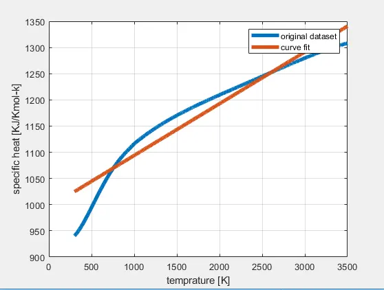
- Use a first-degree polynomial function for the linear fit.
- Now plot to compare original data with curve fit by using linear curve fitting.
- Then give proper labels to the x and y-axis. and add some legend to identify lines.
Plot:
Cubic Fit:
clear all
close all
clc


% loading the data to matlab
cp_data = load('data')
temperature = cp_data(:,1);
cp = cp_data(:,2);

% curve fitting using cubic polynomial
co_efficient = polyfit(temperature,cp,3);
predicted_cp = polyval(co_efficient,temperature);

% plot
plot(temperature,cp,'linewidth',4);
hold on
plot(temperature,predicted_cp,'linewidth',4);
xlabel('temperature [K]')
ylabel('specific heat [KJ/Kmol-K]')
legend('original dataset','curve fit')
grid on
Explanation:
- Start code with the basic command to clear, close, and cancel previous data store in the workspace, command, and editor window. the command uses
- clear all
- close all
- Clc
- Then load the data set using the “load” command into MATLAB for values of temperature and specific heat(Cp).
- Then use the following two functions to perform curve fitting.
- 'Polyfit' is a MATLAB function that computes a least-square polynomial for given data set.polyfit generates the coefficient for the polynomial, which can be used to model a curve to fit the data.
- 'Polyval' evaluates a polynomial for a given set of x values.so, polyval generates a curve to fit the data based on the coefficient found using polyfit.
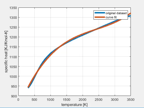
- Use a third-degree polynomial function for the cubic fit.
- Now plot to compare original data with curve fit by using cubic polynomial curve fitting.
- Then give proper labels to the x and y-axis. and add some legend to identify lines.
Plot:
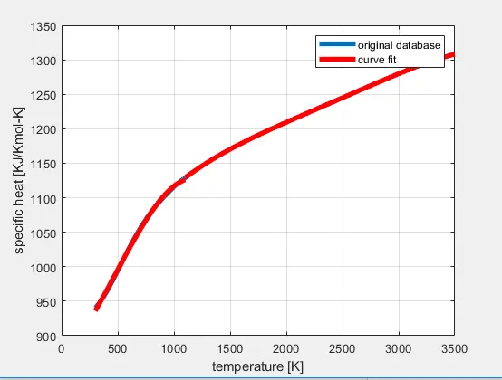
To improve fit or get perfect split the data into small parts. here we convert the given data into 4 equal parts.
Split fit:
clear all
close all
clc


% loading the data to matlab
cp_data = load('data');
temperature = cp_data(:,1);
cp = cp_data(:,2);

%split the data into four part
temperature1 = cp_data(1:800,1);
cp1 = cp_data(1:800,2);

temperature2 = cp_data(801:1600,1);
cp2 = cp_data(801:1600,2);

temperature3 = cp_data(1601:2400,1);
cp3 = cp_data(1601:2400,2);

temperature4 = cp_data(2401:3200,1);
cp4 = cp_data(2401:3200,2);

% curve fitting using cubic polynomial
co_efficient1 = polyfit(temperature1,cp1,3);
predicted_cp1 = polyval(co_efficient1,temperature1);

co_efficient2 = polyfit(temperature2,cp2,3);
predicted_cp2 = polyval(co_efficient2,temperature2);

co_efficient3 = polyfit(temperature3,cp3,3);
predicted_cp3 = polyval(co_efficient3,temperature3);

co_efficient4 = polyfit(temperature4,cp4,3);
predicted_cp4 = polyval(co_efficient4,temperature4);

%plot
plot(temperature,cp,'linewidth',4);
hold on
plot(temperature1,predicted_cp1,'linewidth',4,'color','r');
hold on
plot(temperature2,predicted_cp2,'linewidth',4,'color','r');
hold on
plot(temperature3,predicted_cp3,'linewidth',4,'color','r');
hold on
plot(temperature4,predicted_cp4,'linewidth',4,'color','r');
xlabel('temperature [K]');
ylabel('specific heat [KJ/Kmol-K]');
legend('original database','curve fit')
grid on
Explanation:
- Start code with the basic command to clear, close, and cancel previous data store in the workspace, command, and editor window. the command uses
- clear all
- close all
- Clc
- Then load the data set using the “load” command into MATLAB for values of temperature and specific heat(Cp).
- Split the given data into 4 equal parts.
- Then use the following two functions to perform curve fitting for each split data.
- 'Polyfit' is a MATLAB function that computes a least-square polynomial for given data set.polyfit generates the coefficient for the polynomial, which can be used to model a curve to fit the data.
- 'Polyval' evaluates a polynomial for a given set of x values.so, polyval generates a curve to fit the data based on the coefficient found using polyfit.
- Use a third-degree polynomial function for the cubic fit.
- Now plot to compare original data with curve fit by using cubic polynomial curve fitting.
- Then give proper labels to the x and y-axis. And add some legend to identify lines.
Plot:
Best Fit: It means that the differences between the actual measured values and values predicted by the model equation are minimized.
Perfect Fit: When the curve goes through every point.the sum of square is’0’.and R2 is ‘1’.
How to get the best fit?
- To get best-fit increase the degree of polynomial function till getting the smooth curve fit.
- Split the given data set into small parts to get a closer and fine curve fit.
Conclusion:
In this way, we find the best way to get smooth and goodness of curve fitting using cubic fit and split.
References: