Project 2 - Rankine cycle Simulator

Aim: To create a Rankine cycle simulator using MATLAB.

Objective:

1. Create a code for the Rankine cycle simulator using MATLAB.
2. Plot T-s and h-s plots for given Rankine cycle.
3. Calculate Thermal efficiency, Net-work output, and Back work ratio.

Theory:

RANKINE CYCLE:

• The Rankine cycle is a model used to predict the performance of the steam turbine system.
• The Rankine cycle is an ideal Thermodynamic cycle of a heat engine that converts heat into mechanical work while undergoing a phase change.
• It is an idealized cycle in which the friction losses in each of the four component is neglected.
• The heat is supplied externally to a closed loop, which usually uses water as the working fluid.

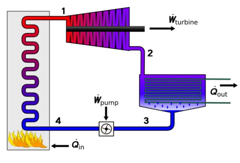
There are four processes in the Rankine cycle.

Process 1-2:

• Isentropic Expansion in the turbine.
• It means the dry saturated vapour expands through a turbine, generating power. This decreases the pressure and temperature of the vapour, and some condensation may occur.

Process 2-3:

• Constant Pressure Heat Rejection by the Condenser.
• The wet vapour then enters a condenser, where it is condensed at a constant pressure to become a saturated liquid.

Process 3-4:

• Isentropic Compression in the feed pump.
• The working fluid is pumped from low to high pressure. As the fluid is a liquid at this stage, the pump requires little input energy.

Process 4-1:

• Constant Pressure Heat Addition by the Boiler.
• The high-pressure liquid enters a boiler, where it is heated at constant pressure by an external heat source to become a dry saturated vapour.

Thermodynamic Equation:

The thermal efficiency of the Rankine cycle is calculated by,

• Thermal efficiency = W_net/Q_in ;

Net-Work Done can be written as,

• W_net = W_pump + W_turbine ;

Work done by the turbine and pump can be written as,

• W_turbine = h₁-h₂ ;
• W_pump = specific volume*(p₁-p₂)*100 ;

Work Back Ratio can be calculated by,

• Work Back Ratio = W_pump/W_turbine ;

Heat supplied in the boiler and heat rejected by the condenser is,

• Q_{in =} h₁-h₄ ;
• Q_out = h₂-h₃ ;

Specific Steam Consumption (SSC) is given as,

• SSC = 3600/W_net ;

Commands:

To get the required output we have to use a specific command which is in-build in MATLAB, so for this particular project we some command which are,

1. disp : This command is used to display the value of a variable.
2. input : This command is used to request user input.
3. XSteam : This function is used to get the required data from the XSteam file.
4. linspace : This command is used to generates an equally and linearly spaced vector.
5. for-loop : This command is used to repeat the loop for a specified number of times.
6. plot : This command is used to plot a 2-D line plot.
7. text : This command is used to add a text description to the data point.
8. axis : This command is used to set axis limits and aspect ratio.
9. xlabel: This command is used to label the x-axis.
10. ylabel: This command is used to label the y-axis.
11. title : This command is to add the title to the plot.
12. legend : This command is used to add a legend to axes.

Code:

clear all
close all 
clc

% display title and processes
disp('                                  RANKINE CYCLE SIMULATOR')
disp('Process 1-2: Isentropic Expansion in the turbine')
disp('Process 2-3: Constant Pressure Heat Rejection by the Condenser')
disp('Process 3-4: Isentropic Compression in the feed pump')
disp('Process 4-1: Constant Pressure Heat Addition by the Boiler')

% Inputs for the given 'RANKINE CYCLE'
p1 = input('Enter the pressure at the turbine inlet (bar) = ');
t1 = input('Enter the temperature at the turbine inlet (Degree celsius) = ');
p2 = input( 'Enter the pressure at the condenser inlet (bar) = ');

% State variables 1
h1 = XSteam('h_ pt',p1,t1);
s1 = XSteam('s_pt',p1,t1);
tsat = XSteam('tsat_p',p1);

% State variables 2
% Since it is isentropic expansion.
s2 = s1; 
% entropy in super-heated region 
sv2 = XSteam('sv_p',p2);

% entropy in sub-cooled region 
sl2 = XSteam('sl_p',p2);

% entropy in wet region
slv2 = sv2-sl2;


% to calculate the dry fraction 
X2 = (s2-sl2)/slv2;

% Enthalpy in super-heated region 
hv2 = XSteam('hv_p',p2);

% Enthalpy in sub-cooled region
hl2 = XSteam('hl_p',p2);

% Enthalpy in wet region
hlv2 = hv2-hl2;

% to calculate Enthalpy
h2 = hl2+(X2*hlv2);

% to calculate temperature 
t2 = XSteam('tsat_p',p2);

% state variable 3
% to calculate temperature 
t3 = t2;      % temerature is constant at process 2-3

% due to Constant Pressure Heat Rejection at process 2-3
p3 = p2;

% to calculate enthalpy
h3 = XSteam('hl_p',p3);

% to calculate entropy
s3 = XSteam('sl_p',p3);

% to calculate specific volume
sp_vol = XSteam('vl_p',p3);

% calculate work-done by the pump
W_pump = sp_vol*(p1-p2)*100;

% calculate work-done by the turbine
W_turbine = h1-h2;

% state variable 4

% due to Constant Pressure Heat Addition by the boiler
p4 = p1;

% to calculate entalpy
% use [W_pump = (h4-h3)]
h4 = W_pump + h3;

% to calculate Entropy
s4 = s3;

% to calculate heat capacity at constant pressure
cp = XSteam('cp_ps',p4,s4);

% to calculate   heat capacity at constant pressure
cv = XSteam('cv_ps',p4,s4);

% to calculate heat capacity ratio
gamma = cp/cv;

% to claculate temperature 
t4 = t3*((p4/p3)^(gamma-1)/gamma);

% state variable 5
t5 = tsat;
h5 = XSteam('hL_p',p1);
s5 = XSteam('sL_p',p1);

% state variable 6 
t6 = t1;
h6 = XSteam('hV_p',p1);
s6 = XSteam('sV_p',p1);

% TO calculate the net-work produced in the cycle
W_net = W_turbine + W_pump;

% to calculate Back Work Ratio
Back_Work_Ratio = W_pump/W_turbine;

% Heat supplied in the boiler
Q_in = h1 - h4;

% Heat rejected by the condenser 
Q_out = h2 - h3;

% Thermal efficiency of the given Rankine Cycle
thermal_eff = W_net/Q_in;

% Specific Steam Consumption (SSC)
SSC = 3600/W_net;

% to get T-S Diagram
% calculate saturation curve point
t = linspace(0,374,1000);

for i = 1:length(t)
    sl(i) = XSteam('sL_t',t(i));
    hl(i) = XSteam('hL_t',t(i));
    sv(i) = XSteam('sV_t',t(i));
    hv(i) = XSteam('hV_t',t(i));
end

% plotting T-S diagram
figure(1)
hold on
grid on
plot(sl,t,'color','b');     % saturated liquid curve
plot(sv,t,'color','r');     % saturated vapour curve
plot([s1 s2],[t1 t2],'color','m');  % plotting work obtained in the turbine
text(s1,t1,'state 1')
plot([s2 s3],[t2 t3],'color','y');  % Plotting heat rejection in the condenser
text(s2,t2,'state 2')
plot([s3 s4],[t3 t4],'color','g');  % Plotting workdone by the pump.
text(s3,t3,'state 3')
plot([s4 s5],[t4 t5],'color','c');  % Plotting the sensible heating process 
text(s4,t4,'state 4')
plot([s5 s6],[t5 tsat],'color','k'); % Plotting latent heating process 
text(s5,t5,'state 5')
plot([s6 s1],[tsat t1],'color','y'); % Plotting the superheating process of steam
text(s6,tsat,'state 6')
axis([0 8 10 500])
xlabel('Enthalpy (KJ/Kg)')
ylabel('Temperature (Degree celsius)')
title ('Temperature vs Enthalpy (T-s) diagram')
legend('saturated liquid curve','saturated vapour curve','work obtained in the turbine','heat rejection in the condenser','workdone by the pump',' sensible heating process','latent heating process',' superheating process of steam','location','northwest')

figure(2)
grid on
hold on
plot(sl,hl,'color','b')             % Saturated liquid curve
plot(sv,hv,'color','r')             % Saturated vapour curve
plot([s1 s2],[h1 h2],'color','m')   % Process 1-2
text(s1,h1,'state 1')
plot([s2 s3],[h2 h3],'color','g')   % Process 2-3
text(s2,h2,'state 2')
plot([s3 s4],[h3 h4],'color','y')   % Process 3-4
text(s3,h3,'state 3')
plot([s4 s1],[h4 h1],'color','k')   % Process 4-1
text(s4,h4,'state 4')
axis([0 8 0 4000])
xlabel('Entropy (KJ/Kg K)')
ylabel('Enthalpy (KJ/Kg)')
title ('Enthalpy vs Entropy (h-s) diagram')
legend('Saturated liquid curve','Saturated vapour curve','Process 1-2','Process 2-3','Process 3-4','Process 4-1','location','northwest')

% print all results

fprintf(                              'RESULT\r\n')

% At State 1
fprintf('At state point 1:\r\n')
fprintf('Pressure at the turbine inlet (P1) = %f bar\r\n',p1)
fprintf('Temperature at the turbine inlet (T1) = %f Deg celcius\r\n',t1)
fprintf('Enthalpy at the turbine inlet (H1) = %f KJ/Kg\r\n',h1)
fprintf('Entropy at the turbine inlet (S1) = %f KJ/Kg-K\r\n',s1)
  

% At State 2
fprintf('At state point 2:\r\n')
fprintf('Pressure at condenser inlet (P2) = %f bar\r\n',p2)
fprintf('Temperature of steam at condenser inlet (T2) = %f Deg.celsius\r\n',t2)
fprintf('Enthalpy of steam at condenser inlet (H2) = %f KJ/Kg\r\n',h2)
fprintf('Entropy of steam at condenser inlet (S2) = %f KJ/Kg K\r\n',s2)
fprintf('Dryness fraction of steam (X2) = %f\r\n',X2)

% At State 3 
fprintf('At state point 3:\r\n')
fprintf('Pressure at the feed water pump inlet (P3) = %f bar\r\n',p3)
fprintf('Temperature at the feed water pump inlet (T3) = %f Deg.celsius\r\n',t3)
fprintf('Enthalpy of water at feed pump inlet (H3) = %f KJ/Kg\r\n',h3)
fprintf('Entropy of water at feed pump inlet (H3) = %f KJ/Kg K\r\n',s3)

% At State 4
fprintf('At state point 4:\r\n')
fprintf('Pressure of water at the boiler inlet (P4) = %f bar\r\n',p4)
fprintf('Temperature of water at the boiler inlet (T4) = %f Deg.celsius\r\n',t4)
fprintf('Enthalpy of water at the boiler inlet (H4) = %f KJ/Kg\r\n',h4)
fprintf('Entropy of water at the boiler inlet (S4) = %f KJ/Kg K\r\n',s4)

% Outputs
fprintf('Thermal efficiency = %f\r\n',thermal_eff)
fprintf('Net work output (W_net) = %f KJ/Kg\r\n',W_net)
fprintf('Back work ratio = %f\r\n',Back_Work_Ratio)
fprintf('Specific steam consumption = %f Kg/KJ\r\n',SSC)

Explanation:

• Start the code with basic command clear all, close all, and clc to clear, close, and cancel all data which previously stored in the workspace, command, and editor window.
• Display the title and processes using ‘disp’ command.
• Using the ‘input’ command gives the inputs to the given problem which show in the command window, after that you can able to give inputs in the command window to get desired results.
• To calculate all state variables use “XSteam” file, as a function to extract all values of state variables.

State variable 1:

• There are three unknown variables at state 1 which are ‘saturated temperature (t_sat), enthalpy (h₁), entropy (s₁)’.
• Pressure(p₁) is given as pressure at turbine inlet is ‘30 bar’ and Temperature(t₁) at the turbine inlet is ‘400 deg.Celcius’.
• To calculate the state variable at state 1 use ‘XSteam’ function. As we know the values of ‘p₁’ & ‘t₁’ we can find all variables with help of that.

State variable 2:

• Since there is an isentropic expansion, Entropy s₂ = s_1.
• To calculate dryness fraction we have to calculate entropy at super-heated (sv₂), entropy at sub-cooled region (sl₂), and entropy at wet region (slv₂) from ‘XSteam’ file with pressure (p₂) as a known variable.
• To calculate Enthalpy (h₂) we have to calculate enthalpy at super-heated region(hv₂), enthalpy at sub-cooled region (hl₂), and enthalpy at wet region (hlv₂) from ‘XSteam’ file with pressure (p₂) as a known variable.
• Here temperature (t₂) = saturated temperature (t_sat).

State variable 3:

• Due to Constant Pressure Heat Rejection at the process, pressure ‘p₃ = p_2’ and temperature ‘t₃ = t₂’.
• Calculate the Enthalpy (h₃) and Entropy (s₃) from ‘XSteam’ file with pressure( p₃) as a known variable.
• Calculate Specific volume (sp_vol) to calculate Work done by the pump (W_pump).
• Calculate Work done by the turbine (W_turbine) equation (h₁-h₂).

State variable 4:

• Due to Constant Pressure Heat Addition by the boiler at the process, pressure ‘p₄ = p₁’ and entropy ‘s₄ = s₃’_.
• Calculate Enthalpy (h₄) by equation (W_pump + h₃).
• To calculate Temperature (t₄) we have to calculate heat capacity at constant pressure (c_p) and heat capacity at constant pressure from ‘XSteam’ with pressure (p₂) and entropy (s₄). After that calculate the heat capacity ratio.

State variable 5:

• At state 5 we are at a saturated liquid phase so ‘t₅ = t_sat’.
• Calculate Enthalpy (h₅) and Entropy (s₅) for the saturated liquid phase from ‘XSteam’ with pressure (p₁).

State variable 6:

• At state 6 temperature ‘t₆ = t₁’.
• Calculate Enthalpy (h₆) and Entropy (s₆) for the saturated vapour phase from ‘XSteam’ with pressure (p₁).

To calculate results:

• Calculate net-work produced in the cycle, Back work ratio, heat supplied in the boiler,
• Heat rejected by the boiler, Thermal efficiency of the given Rankine cycle, and Specific Steam Consumption using given formulae.

Plot:

T-s plot:

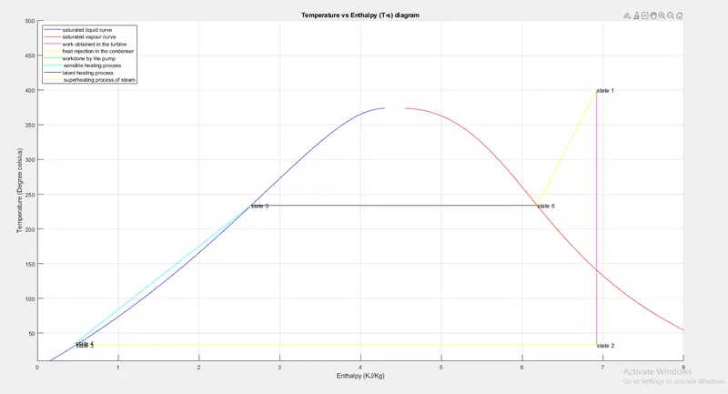
• To get the saturated liquid curve and saturated vapour curve we have to use ‘for-loop’. We use the values of Enthalpy and Entropy for the saturated liquid phase and saturated vapour phase.
• And with the help of ‘linspace’ we generate the equally space vector for temperature.
• Then plot ‘T-s plot’ using appropriate state values of Temperature (t) and Entropy(s) to get an accurate state point.
• Using the ‘text’ command add a text description to states.
• Using the ‘axis’ command set axis limits and aspect ratio.
• Using the ‘label’ command give labels to the x-axis and y-axis.
• Using the ‘title’ command give the title to the plot.
• Using the ‘legend’ command adds a legend to axes.

h-s plot:

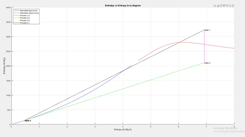
• Then plot ‘h-s plot’ using appropriate state values of Enthalpy (h) and Entropy(s) to get an accurate state point.
• Using the ‘text’ command add a text description to states.
• Using the ‘axis’ command set axis limits and aspect ratio.
• Using the ‘label’ command give the label to the x-axis and y-axis.
• Using the ‘title’ command give the title to the plot.
• Using the ‘legend’ command adds a legend to axes.

Print results and output:

• To print all state results and output use ‘fprintf’ command.

Plot:

T-s plot:

h-s plot:

Result:

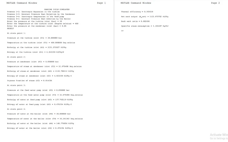
• This is the result of the Rankine cycle simulator. The original pdf file is attached to the challenge browse window.

Error:

• During creating code there is some mathematical error occurs. to overcome that I put the appropriate values for the equation.
• I don't face any command related errors.

Conclusion:

• In this way,we find the Thermal efficiency = 36.36 %, Back Work Ratio = 0.0027, and Net Work Output = 1123.87 KJ/Kg.

References:

• https://en.wikipedia.org/wiki/Rankine_cycle.
• https://www.youtube.com/watch?v=XB55LQ12ScI