Understanding Genetic Algorithm using MATLAB
Week-4 Report.
- Aim: To write a code that executes a Genetic Algorithm and calculates the Maximum value of the given function.
- Introduction:
A genetic algorithm (GA) is a method for solving both constrained and unconstrained optimization problems based on a natural selection process that mimics biological evolution. The algorithm repeatedly modifies a population of individual solutions. At each step, the genetic algorithm randomly selects individuals from the current population and uses them as parents to produce the children for the next generation. Over successive generations, the population "evolves" toward an optimal solution.
We can apply the genetic algorithm to solve problems that are not well suited for standard optimization algorithms, including problems in which the objective function is discontinuous, nondifferentiable, stochastic, or highly nonlinear.
The genetic algorithm differs from a classical, derivative-based, optimization algorithm in two main ways, as summarized in the following table.
| Classical Algorithm | Genetic Algorithm |
|---|---|
| Generates a single point at each iteration. The sequence of points approaches an optimal solution. | Generates a population of points at each iteration. The best point in the population approaches an optimal solution. |
| Selects the next point in the sequence by a deterministic computation. | Selects the next population by computation which uses random number generators. |
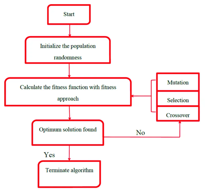
Overview of the Genetic Algorithm
- Code/Logic:
1. We firstly need to clear and close all the previously entered codes and the present values of the already used variables, hence we use the following commands:
clear all
close all
clc
2. We start the code by stating the first Study case and the conditions that we have applied to it. In the first study case, we do not have the Lower and Upper Bounds and the control over the population.
So, in this case, the sampling will also be very random and not within the bounds that we expect. To begin with the code, we start by mentioning the search space, that is, the x and y values. We also need to mention the number of iterations or the number of times that we will run the code. In this step, we will also define a seperate function that we can use for the plot.
3. From the array that we made in the above step, we will create a matrix by using the meshgrid command.
4. In the next step, we will define a for loop that will run the genetic algorithm function for the number of times we want the code to run, i.e. the number of iterations for the code. The for loop is running a different function that have defined in a completely different script. From this function, we have taken two outputs, i.e the co-ordinates at which we get the maximum value.
5. So, in general, the Genetic Algorithm is suppposed to return the minimum value for the function that we give as input. So, since we require the maximum value from the defined function, we simply extract a negative value for the function and then plot the absolute or the mod of this value. Like this, we can extract the maximum value of the function.
6. The syntax that we use for the Genetic Algorithm are as follows:
%Syntax for the Genetic Algorithm function:

x = ga(fun,nvars)
x = ga(fun,nvars,A,b)
x = ga(fun,nvars,A,b,Aeq,beq)
x = ga(fun,nvars,A,b,Aeq,beq,lb,ub)
x = ga(fun,nvars,A,b,Aeq,beq,lb,ub,nonlcon)
x = ga(fun,nvars,A,b,Aeq,beq,lb,ub,nonlcon,options)
x = ga(fun,nvars,A,b,[],[],lb,ub,nonlcon,IntCon)
x = ga(fun,nvars,A,b,[],[],lb,ub,nonlcon,IntCon,options)
x = ga(problem)
[x,fval] = ga(___)
[x,fval,exitflag,output] = ga(___)
[x,fval,exitflag,output,population,scores] = ga(___)
All these methods of writing the Genetic Algorithm have its own meaning and different purposes. So, if we have to specify the population size, or even the upper and the lower bounds for the function, we have to use this syntax appropriately according to its own meaning.
7. In the last step for this case, we simply plot the results of the various outputs that we have requested. To plot more than one plot in the same figure window, we use the subplot command. In this command, we can plot different plots under the same figure window and study the properly.
So the Basic syntax for the subplot, is subplot(m,n,p) where :
m = Number of Grid rows
n = Number of Grid Columns
p = Grid position for new Axes.
Another command that we used is the surfc command. This command creates a three-dimensional surface plot with a contour plot underneath
8. Plot3 command is used to plot a 3D plot between three variables. We must label the axez properly as well.
Like this we can run the first study and then study the plots if needed.
9. Similar to the first case, we will create a new code to plot for the second study. in the second Study, we simply have to add an upper and a lower bound or limit for the function to run. Doing this we are able to limit the number of different outputs that we get in the same number of iterations. It helps us concise the results and study the function behaviour only in a specific limit.
To add the lower and upper bounds, we simply have to change the input definition of the genetic algorithm according to its syntax. In pur case, the lower and upper limits have been set to 0 to 0.6 in both the x and y axis. We then plot the results for this and see that the maximum value for the function is changing in a much smaller range.
10. To increase the accuracy of the function output, we can increase the population size for the function, and this is precisely our study3. So, if the number of independent variables in the function is less than or equal to 5, then the solver takes the population size to be 50 or else 200. In our case, the number of Independent variables is 2, hence by default the population size is 50, but since we want to increase the population size, will use the optim command.
11. So to change the population size, we specify a variable that stores the changed population size Genetic Algorithm settings. We then use this variable to then define the population size of the defined Genetic Algorithm function. We have kept the population size to 300. The only down side to increasing thepopulation size from 50 to 300 is that it increases the GA command run time.
The Main Code for all the three cases is as follows:
clear all close all clc %Study1: Without constraints and population control. %Defining search space x = linspace(0,0.6,150); y = linspace(0,0.6,150); n = 50; %Number of Iterations to be run f = get_stalagmite(x,y); %creating 2D Mesh [xx,yy] = meshgrid(x,y); tic %Evaluating the stalagmite function for i =1:n; [inputs, fopt(i)] = ga(@stalagmite,2); xopt(i) = inputs(1); yopt(i) = inputs(2); end study1_time = toc figure (1) subplot (2,1,1) hold on surfc(xx,yy,f) shading interp title ('Unbounded inputs') plot3(xopt, yopt, abs(fopt),'marker', 'o', 'markersize', 5, 'markerfacecolor','r') subplot(2,1,2) plot (abs(fopt)) xlabel('Iterations') ylabel('Function Maximum') %Study2:With Upper and Lower bounds: %Defining search space x = linspace(0,0.6,150); y = linspace(0,0.6,150); n = 50; %Number of Iterations to be run f = get_stalagmite(x,y); %creating 2D Mesh [xx,yy] = meshgrid(x,y); tic %Evaluating the stalagmite function for i =1:n; [inputs, fopt(i)] = ga(@stalagmite, 2, [], [],[],[], [0;0],[0.6;0.6]); xopt(i) = inputs(1); yopt(i) = inputs(2); end study2_time = toc figure (2) subplot (2,1,1) hold on surfc(xx,yy,f) shading interp title ('Bounded Inputs') plot3(xopt, yopt, abs(fopt),'marker', 'o', 'markersize', 5, 'markerfacecolor','r') subplot(2,1,2) plot (abs(fopt)) xlabel('Iterations') ylabel('Function Maximum') %Study3: With upper and lower bounds and population size control options = optimoptions ('ga'); options1 = optimoptions (options, 'PopulationSize', 300); tic %Evaluating the stalagmite function for i =1:n; %n =Number of Iterations to be run [inputs, fopt(i)] = ga(@stalagmite,2,[],[],[],[], [0;0],[0.6;0.6], [], [], options1); xopt(i) = inputs(1); yopt(i) = inputs(2); end study3_time = toc figure (3) subplot (2,1,1) hold on surfc(xx,yy,f) shading interp title ('Bounded Inputs w Population control') plot3(xopt, yopt, abs(fopt),'marker', 'o', 'markersize', 5, 'markerfacecolor','r') subplot(2,1,2) plot (abs(fopt)) xlabel('Iterations') ylabel('Function Maximum') %end
Since we have defined two functions, the code for them are as follows:
a. Staglamite function:
%Staglamite_function function f = stalagmite(input) x = input(1); y = input(2); term1 = (sin(5.1*pi*x + 0.5)).^6; term2 = (sin(5.1*pi*y + 0.5)).^6; term3 = exp(-4*log(2)*(x-0.0667).^2 / (0.64)); term4 = exp(-4*log(2)*(y-0.0667).^2 / (0.64)); f = -(term1 * term2 * term3 * term4); end
b . Get_staglamite Function:
%get_staglamite_function function f = get_stalagmite (x,y) [xx,yy] = meshgrid(x,y); term1 = (sin(5.1*pi*xx + 0.5)).^6; term2 = (sin(5.1*pi*yy + 0.5)).^6; term3 = exp(-4*log(2)*(xx-0.0667).^2 / (0.64)); term4 = exp(-4*log(2)*(yy-0.0667).^2 / (0.64)); f = (term1 .* term2 .* term3 .* term4); end - Results:
The Plots for all the Simulations are attached below:
Study1: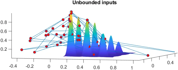
Case1 3D plot.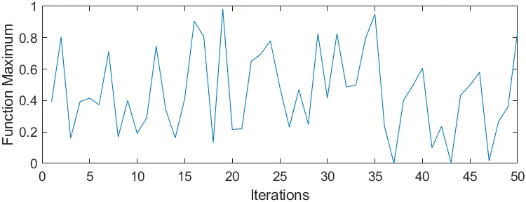
Case1 Iterations v Maxima plot
Study2: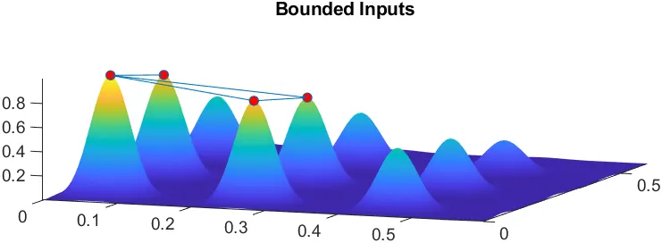
Case2 3D plot.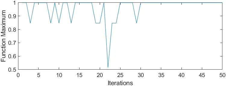
Case2 Iterations v Maxima plot
Study3: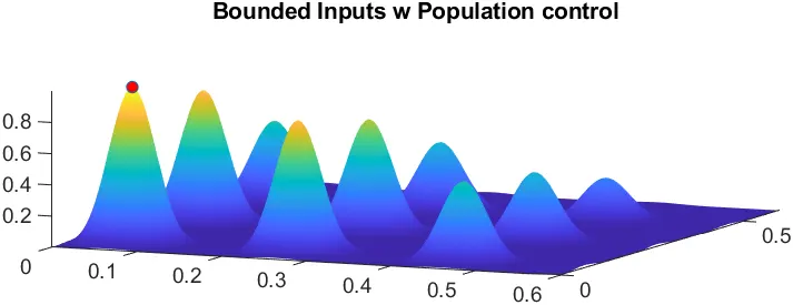
Case3 3D plot.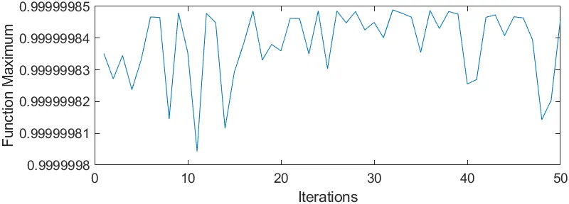
Case3 Iterations v Maxima plot
As we can clearly see that the plot in the first study is much more chaotic and not accurate at all. It gives a different Function maxima for every iteration. It simply means that the algorithm is taking a random sample for every iteration and hence the results are scattered all over the graph.
In the second study, the results are much more concise and within a small range as well. In this case, since we have put an upper and lower bound to the sampling, the results are much more accurate for the function as well.
In the third study, the value of the function maxima varies between 0.99999985 and 0.99999981 which is pratically a straight line if we zoom out from the plot. This happened because in the third study, we have put the lower and upper bounds and also increased the Population size. Increasing the population size will increase the run time for the algorithm but will also increase the accuracy of the algorithm. - Errors: The errors that I faced were majorly the typos and the parantheses while using specific commands. So, when MATLAB pointed out an error, I checked for the line number and then checked for any typos and corrected them right away.
- Conclusion: In conclusion, I would like to state that this challenge helped me understand how the Genetic Algorithm works and how to increase the accuracy of the plots as well.