Week 4 - Genetic Algorithm

Aim - To Optimize the stalagmite function to find global maxima using genetic algorithm.

Theory -

Genetic Algorithm (GA) is a search-based optimization technique based on the principles of Genetics and Natural Selection. It is frequently used to find optimal or near-optimal solutions to difficult problems which otherwise would take a lifetime to solve. It is frequently used to solve optimization problems, in research, and in machine learning.Genetic Algorithm (GA) is a search-based optimization technique based on the principles of Genetics and Natural Selection. It is frequently used to find optimal or near-optimal solutions to difficult problems which otherwise would take a lifetime to solve. It is frequently used to solve optimization problems, in research, and in machine learning.

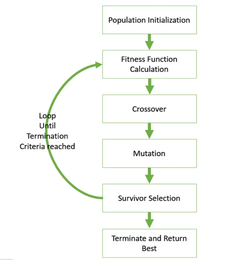
Flowchart for the Genetic algorithm -

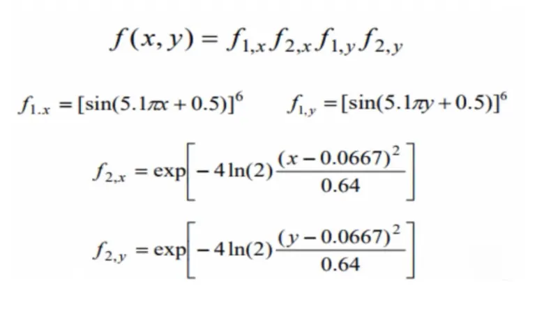
Input function -

Following is the input function for the input

Genetic Algorithm Syntax in MATLAB -

[x,fvar,exitflag,output,population,scores] = ga(func,nvars,A,b[],[],lb,ub,nonlcon,lntcon,options)

Where,

x = optimum solution

exitflag = reason ga stopped

output = information about optimization process

population = final population

scores = final scores

fun = fitness function

nvars = number of variables

A,b = Linear inequality constraints

Aeq,beq = Linear equality constraints

lb = Lower bound

ub = Upper bound

nonlcon = Use for nonlinear constraints

lntCon = To get solution in integer

options = To set population size minimize with non default options

Stalagmite function -

1. The function is created and its input vector is specified.

2. The equation is then substituted as variables f1,f2,f3,f4 and the combined to form final output variable f.

3. Negative sign specifies that we need maxima for the corressponding equation.

Stalagmite function code -

function [f]=stalagmite(input_vec)

x = input_vec(1);
y = input_vec(2);

f1 = (sin(5.1*pi*x + 0.5)).^6;
f2 = exp(-4.*log(2)*((x-0.0667).^2)./(0.64));
f3 = (sin(5.1*pi*y + 0.5)).^6;
f4 = exp(-4.*log(2)*((y-0.0667).^2)./(0.64));

f = -(f1*f2*f3*f4);
end

Genetic Algorithm for stalagmite function -

1. Linspace command is used to to create x and y array with 150 elements between 0 to 0.6.

2. The variable 'rep' is defined that sets no of iterations to 50.

3. A 2D grid is created using meshgrid from x and y which is stored in variables xx and yy.

4. For loop is used to solve genetic algorithm for every element in that 2D mesh with length of rows and columns used as counter.

5. Then the input vector is declared as ga requires an input vector to store each value in mesh grid.

6. Tic command is used to start timer.

7. For loop constrained with number of iteration is formed to run ga for unbound statistical [Study 1].

8. The smallest value for each iteration is obtained and its coordinates are stored in seperate variable.

9. Figure 1 is plotted by using subplot command to partition the plot window to get more than one plots window. one column and 2 rows are specified and then position of each plot is selected.

10. The surfc command is used to plot contour with xx and yy value from mesh grid as input and negative optimum value is used to get maxima of function.

11. Shading interp is used to smoothen the function plot and remove grid lines.

12. Then the plot3 command is used to create 3D plot of x y and negative fopt to get maxima of function.

13. The same Study is repeated with bounded ga.

14. Further study includes introduction of optim option to improve accuracy which increases the poplulation size.

Code -

clear all
close  all
clc

x = linspace(0,0.6,150);
y = linspace(00,0.6,150);

% Convertion 1D array to 2D array
[xx yy] = meshgrid(x,y);
rep = 50;                   % No. of iterations

tic

for i = 1:length(xx)
    for j = 1:length(yy)
        
        input_vec(1) = xx(i,j);
        input_vec(2) = yy(i,j);
        f(i,j) = stalagmite(input_vec);
        
        end
end

study_time = toc

surfc(xx,yy,-f)
shading interp
xlabel('x value')
ylabel('y value')
title('stalagmite function')


% Study - 1

tic

for i = 1:rep
    [inputs,fopt(i)] = ga(@stalagmite,2);
    xopt(i) = inputs(1);
    yopt(i) = inputs(2);
end

study_time1 = toc

figure(1)
subplot(2,1,1)
hold on
surfc(x,y,-f)
shading interp
plot3(xopt,yopt,-fopt,'Marker','o','MarkerSize',5,'MarkerFaceColor','r')
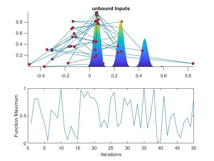
title('unbound Inputs')
subplot(2,1,2)
plot(-fopt)
xlabel('Iterations')
ylabel('Function Maximum')


% Study - 2

tic

for i = 1:rep
    [inputs,fopt(i)] = ga(@stalagmite,2,[],[],[],[],[0;0],[0.6;0.6]);
    xopt(i) = inputs(1);
    yopt(i) = inputs(2);
end

study_time2 = toc

figure(2)
subplot(2,1,1)
hold on
surfc(x,y,-f)
shading interp
plot3(xopt,yopt,-fopt,'Marker','o','MarkerSize',5,"MarkerFaceColor",'r')
title('Optimum Solution')
subplot(2,1,2)
plot(-fopt)
xlabel('Iterations')
ylabel('Function Maximum')

% Study - 3

options = optimoptions(@ga)
options = optimoptions(options,'PopulationSize',170);

tic
for i = 1:rep
    [inputs,fopt(i)]=ga(@stalagmite,2,[],[],[],[],[0;0],[1;1],[],[],options);
    xopt(i) = inputs(1);
    yopt(i) = inputs(2);
    
end

study_time3 = toc

figure(3)
subplot(2,1,1)
hold on
surfc(x,y,-f)
shading interp
plot3(xopt,yopt,-fopt,'Marker','o','MarkerSize',5,"MarkerFaceColor",'r')
title('Optimum Solution')
subplot(2,1,2)
plot(-fopt)
xlabel('Iterations')
ylabel('Function Maximum')

global_maxima = -fopt

Result -

1. Unbound solution

2. Bound Solution

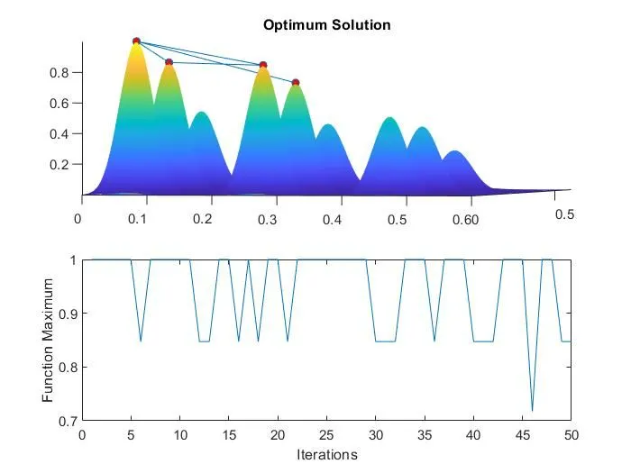
3. Optimum Solution

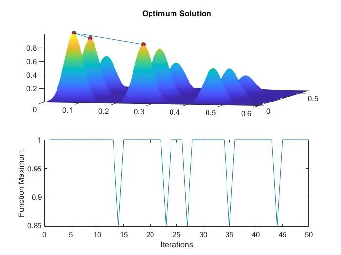
Global Maxima = 1