Week 3 - Solving second order ODEs

Aim - To Solve the ODE for the Simple Harmoic motion of a simple pendulum and create an animation of motion of pendulum

Inputs -

lenght of string = l =1m

mass of pendulum = m = 1kg

damping coefficient = b = 0.05

gravity = g = 9.81 m/s^2

Theory - A simple pendulum consists of a point mass attached to a string suspended downwards.

The motion of swinging of a pendulum about its mean position is know as Simple harmonic motion (S.H.M).

The motion of the pendulum is governed by follow differential equation,

Methodology

1. Function to solve ODE -

A function is created to simplify the ODE to a 1st order differential equation in order for the solver ode45 to solve it

following is the code for the function,

function [dtheta_dt] = ode_f(t,theta,b,g,l,m)

% Solving 2nd oder ODE 
theta1 = theta(1);
theta2 = theta(2);

dtheta1_dt = theta2;
dtheta2_dt = -(b/m)*theta2 - (g/l)*sin(theta1);
dtheta_dt = [dtheta1_dt; dtheta2_dt];
end

2. Solving ODE and animation

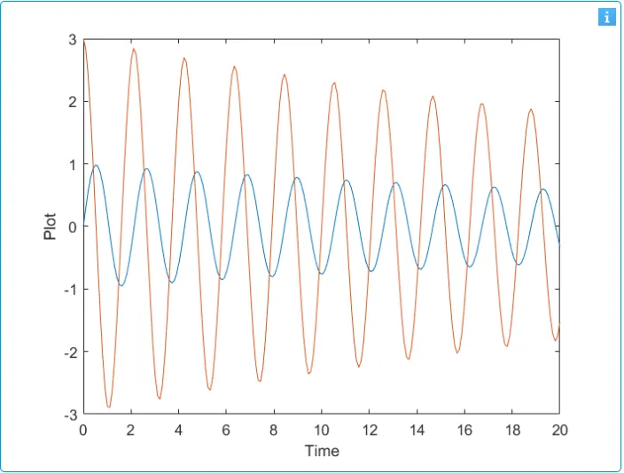
Time span of oscillation is set using linspace array from 0 to 20 s with 200 divisions

Ode is solved using the solver ode45 and call the above mentioned function

Oscillation is plotted on graph using plot command

To get frames for the oscillation of the pendulum for loop is used

Polar coordinates of the circular motion of the ball is converted to geometric coordinates

Animation is generated using movie command in matlab

Flollowing is the code,

clear all
close all
clc


% Solving Pendulum oscillation 2nd order ODE 

% Inputs

b = 0.05;
g = 9.81;
m = 1;
l = 1;

% Initial conditions
theta_0 = [0;3];

% Time period
t_span = linspace(0,20,200);
 
% Solving ODE
[t,result] = ode45(@(t,theta) ode_f(t,theta,b,g,l,m), t_span, theta_0);

% Plotting graph

plot(t,result (:,1))
hold on 
plot(t,result (:,2))

xlabel('Time')
ylabel('Plot')

ct = 1
 
% Loop to create oscillation 
for i = 1:length(t)
     
    % initial position
     x0 = 0;
     y0 = 0;
     
    % Final position
     x1 = 1*sin(result(i,1));
     y1 = -1*cos(result(i,1));
    
    % Plot
     figure(2)
     
     % Base line
     plot([-1,1],[0,0],'LineWidth',5,'Color','b')
     
     % Pendulum String
     plot([x0 x1],[y0 y1],'LineWidth',3,'Color','r')
     
     hold on
     
     % Pendulum ball
     plot(x1,y1,'o','markers',30,'MarkerFaceColor','b')
     
     grid on
     axis ([-2 2 -2 1])
     pause(0.01)
     hold off;
     M(ct) = getframe(gcf) ;
     ct = ct + 1;
     
 end

 % Creating Animation
 
 movie(M)
 videofile = VideoWriter('Pendulum_o.avi', 'Uncompressed AVI');
 open(videofile)
 writeVideo(videofile,M)
 close(videofile)

Result

1. Graph

Animation -

https://drive.google.com/file/d/1-eqMPZH-63VU3-4XccfbXDN7ZBgsjvp9/view?usp=sharing