Week-4 Challenge WOT Condition Part-2

AIM :

1. To understand the difference between mapped and dynamic model of engine, motor and generator.
2. Fuel Economy - Miles per gallon and its calculation.
3. Run the HEV ReferenceApplication with WOT drive cycle. Change the grade and wind velocity in the environment block and compare the results.
4. To compare the simulated results of hybrid and pure electric powertrains.

INTRODUCTION :

Powertrain Blockset™ provides fully assembled reference application models of automotive powertrains, including gasoline, diesel, hybrid, and electric systems. It includes a component library for simulating engine subsystems, transmission assemblies, traction motors, battery packs, and controller models. Powertrain Blockset also includes a dynamometer model for virtual testing. MDF file support provides a standards-based interface to calibration tools for data import.

Powertrain Blockset provides a standard model architecture that can be reused throughout the development process. You can use it for design tradeoff analysis and component sizing, control parameter optimization, and hardware-in-the-loop testing. You can customize models by parameterizing components in a reference application with your own data or by replacing a subsystem with your own model.

Key Features

• Fully assembled models of gasoline, diesel, hybrid and electric components.
• Libraries of engine, transmission, traction motor and battery components.
• Basic controllers for powertrain subsystems.
• Standard drive cycle data, including FTP75, NEDC and WOT.
• Engine dynamometer model for virtual calibration and testing.
• MDF file support for calibration data import

1. To understand the difference between mapped and dynamic model of engine, motor and generator.

Powertrain Blockset provides two different types of combustion engine models :

• Mapped
• Dynamic

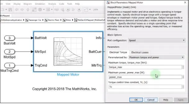
1. Mapped Model :

Mapped engines represents maro engine behaviour as a set of look up tables (Brake Torque, fuel flow, air mass flow, exhaust temperature, efficiency and emissions) as functions of commanded load and measured engine speed. Mapped model is also referred as as a static system.

Mapped engine models are suitable for analysis and design activities that do not require engine subsystem dynamic characteristics, for example in engine and transmission powertrain matching analysis for fuel economy, emissions and performance trade-offs.

2. Dynamic Model :

Dynamic engines decompose engine behaviour into individual component models that account for engine dynamics, most notably intake airflow and turbocharger dynamics.

Dynamic engine models are suitable for designing control, estimator and diagnostic algorithms that depend on dynamic subsystem states for example, in closed loop AFR control algorithm development.

This principle remains same for motor and generator. One can switch between types of engine modes based on application.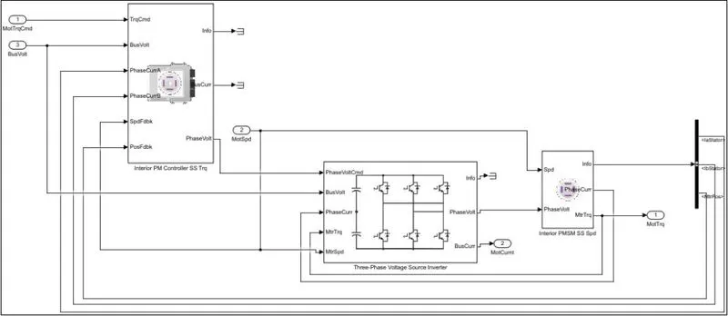

2.Fuel Economy - Miles per gallon and its calculation.

Miles per Gallon (MPG)

Miles per gallon is a fuel economy rating determined by how far a car can travel on a gallonn of gasoline or diesel.

In case of electric vehicles, this can be defined as the amount of distance travelled by the engine powered car per gallon of fuel and compared to the electric energy consumped by an EV to cover the same distance i.e. Equivalent energy consumped to propel the car through same distance.

The powertrain blocksets has the built in model for this,

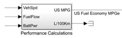
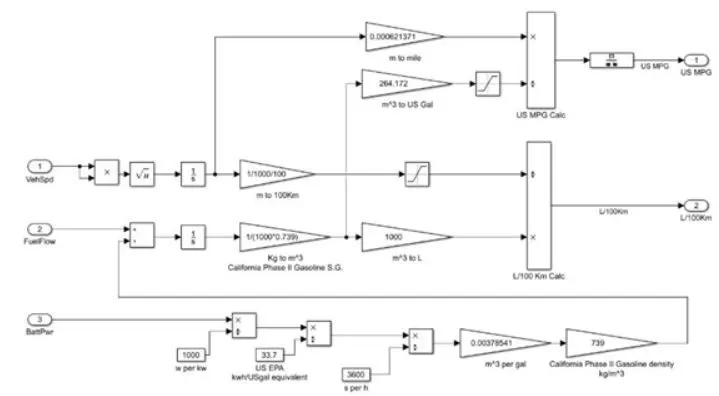
According to the model, following 3 factors are involved in calculating the fuel economy rating,

• Vehicle speed
• Fuel Flow
• Battery Power
• Vehicle Speed is a critical criterion in evaluating the Fuel consumption/Fuel flow.
• Vehicle speed is intergrated with respect to time to obtain distance travelled later which is km units. Saturation block is used to bound upper and lower limits to the obtained value.
• Total Battery Power required to propel the vehicle is simulated along way, Battery Power is converted to 'kW' and Battery Rating is obtained in terms of 'kWh'. Several gains block with some constant values are used to get the mass flow rate of the fuel is (Kg /m^3).
• The above value is fed back as input in the fuel flow block, using these values along with the Gain Blocks fuel consumption in 'litres' is calculated.
• By the results obtained from speed and fuel flow, the total amount of fuel to run vehicle for 100 Km is obtainedd (L/100 Km)
• To evaluate for MPG,

1. Consider the fuel flow value in m^3 and convert it into US Gal by multiplying with 246.172 in gain block and saturate the limits.
2. Simultanously consider the distance travelled in meter and convert to miles using gain block.
3. Now from above two values MPG can be obtained.

3.Run the HEV ReferenceApplication with WOT drive cycle. Change the grade and wind velocity in the environment block and compare the results.

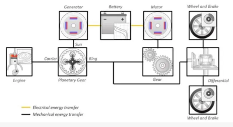
The reference HEV Powertrain Blockset is extracted from MathWorks,

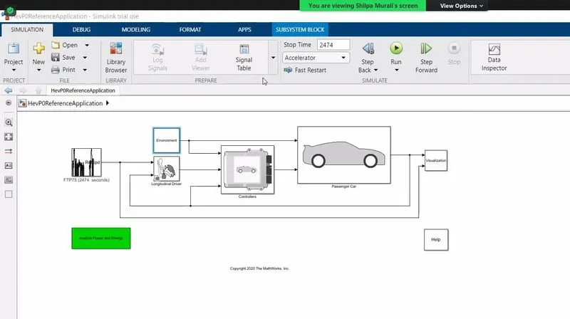
• Drive Cycle Soureblock : Generates a standard or user-specified driver cycle velocity versus the profile. In this simulation we are evaluating for WOT.
• Environment Subsystem : Creates environment variables including road grade, wind velocity and atmospheric temperature and pressure.
• Longitudinal Driver Subsystem : Uses the longitudinal driver or open loop variant to genetrate normalized acceleration and braking commands.

1. Longitudinal Driver variant implements a driver model that uses vehicle target and reference velocities.
2. Open loop variant allows you to configure the acceleration, deccleration, gear, electric plant and engine subsystems.

• Controller Subsystem : Implements a powertrain control module (PCM) containing an input power-split hybrid control module (HCM) and an engine control module (ECM).
• Visualization Subsystem : Displays vehicle-level performance, battery SOC, fuel economy and emission results that are useful for powertrain matching and component selection analysis.

Simulation for WOT_1 :

• Grade Angle = 0 degree
• Wind Velocity = 0 m/s
• Total Simulation Time = 100 s
• Nominal Speed = 50 m/s (WOT Max speed = 180 kmph = 112 Mph)
• Time at decceleration = 50 s

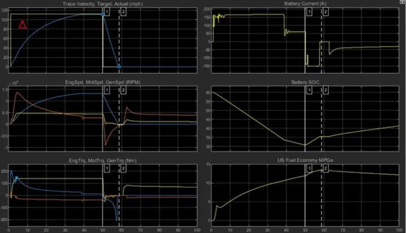
Trace Velocity : A shift/Delta exists between actual and target WOT condition. This can be used to determine the peak speed and to the limitations on the maximum power availability from Energy Sources at that instant.

• Max Velocity is attaind at t = 40 s
• Decceleration Time to 0 Mph = 8.765 s

Speed (RPM) : Displays the speed of engine , motor and generator throughout the simulation. This can be used to determine the peak speed and to correlate between the engine and generator RPM.

Torque (Nm) : A useful Torque Characteristics curve. To achieve the top speed (WOT)

• Max Engine Torque = 140 Nm
• Peak Motor Torque = 200 Nm (Instantaneous during start)

Battery Current (A) :

• Max Current Drawn from battery to achieve WOT = 168 A
• Current drawn after attaining Max. speed = 63 A
• Current during Decceleration = - 141 A

Battery SOC (%) :

• The SOC of Battery decreased from initial 60% to 33.5% rapidly in linear
• ction is reduced once vehicle attains top speed and SOC slowly depletes to 30%.
• During decceleration, battery SOC has increased to 36 % which constitutes regenerative braking.

Simulation for WOT_2 (HEV) :

• Grade Angle = 5 degrees
• Wind Velocity = 10 m/s
• Total Simulation Time = 100 s
• Nominal speed = 50 m/s (WOT Max speed = 180 Kmph = 112 Mph)
• Decceleration time = 50 s

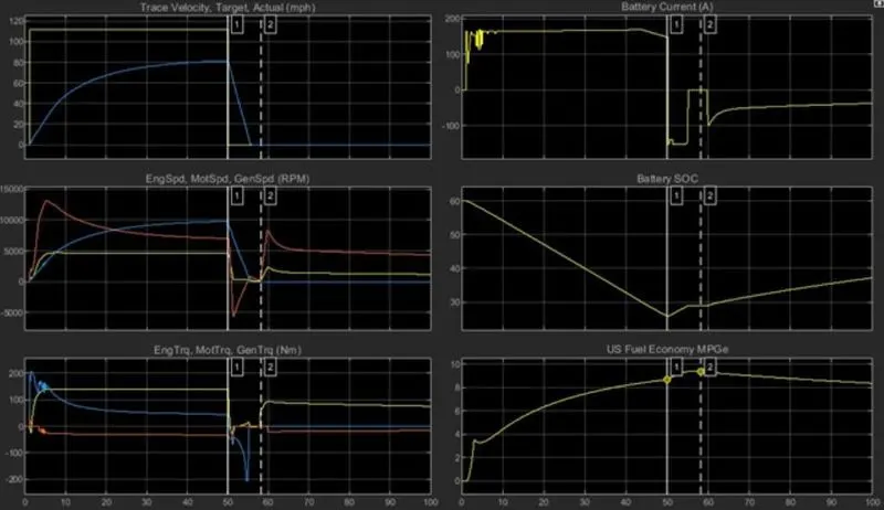
Result Comparison -

	Simulation_1	Simulation_2
Grade Angle (Deg)	0	5
Wind Velocity (m/s)	0	10
Max speed (Mph)	112	86.5
Decceleration time (s)	8.765	5.45
Max Engine Torque (Nm)	140	140
Peak Motor Torque (Nm)	200	200
Max Battery current drawn (A)	168	168
Battery SOC (%)	60 to 30	60 to 25
Fuel Economy (MPG)	13.5	9.2

Conclusion :

• There exists a difference between actual velocity curve and the input curve due to limitations in max. power available from propulsion/energy sources.
• Limiting factors involves current or the battey module.
• The maximum speed is achieved in Simulation_2 is less than Simulation_1 because of the presence of grade angle and opposing wind force.
• It can be observed that with increase in grade angle, WOT response time increases and velocity decreases.
• The battery SOC also decreases considerably with increase in traction force.
• Fuel economy falls to greater extent with increase in the demanding traction power.

4. To compare the simulated results of hybrid and pure electric powertrains.

Following reference models from Mathwork are used for simulation

EV

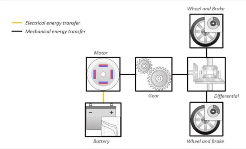
HEV

Simulation for WOT_3 (EV)

• Grade Angle = 5 degree
• Wind velocity = 10 m/s
• Total Simulation Time = 100s
• Nominal Speed = 50 m/s (WOT Max speed = 180 Kmph = 112 Mph)
• Decceleration time = 50s

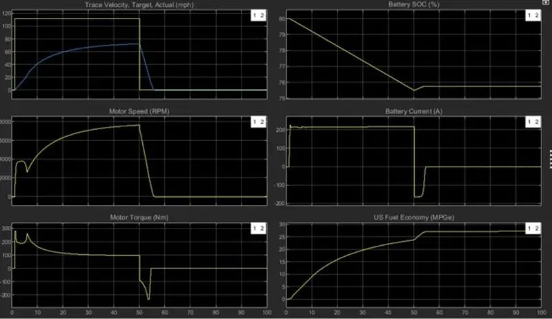
Result Comparison -

	EV	HEV
Grade Angle (Deg)	5	5
Wind Velocity (m/s)	10	10
Max speed (Mph)	72	86.5
Decceleration time (s)	5.8	5.45
Max Engine Torque (Nm)	-	140
Peak Motor Torque (Nm)	280	200
Max Battery current drawn (A)	217	168
Battery SOC (%)	80 to 75.5	60 to 25
Fuel Economy (MPG)	27	9.2

Conclusion :

• The Pure EV drive achieve less Top speed as compared to HEV.
• Motor used in EV must be more powerful than the one used in HEV.
• EV derives all power from motor alone and hence Torque developed by EV motor is greater, whereas in HEV combined torque from motor and engine propels the system.
• The conventional HEV uses Lead Acid Battery whereas EV uses Lithium ion Battery which has more potential.
• Instantaneous torque at the start is more in EV compared to HEV or conventional vehicles.