Week 4 - Genetic Algorithm

GENETIC ALGORITHM

AIM: Write Matlab program to find maxima of a function.

OBJECTIVE: Use genetic algorithm to find global maxima of a stalagmite function.

BODY OF WORK:

A genetic algorithm is used to optimize a function by finding maxima value. In matlab, inbuilt function of genetic algorithm can only find minima, so function will be mirrored about the X-Y plane. The minima of mirrored function will have the same coordinates as maxima of original function. Genetic algorithm function in matlab starts with an initial population of parent individual solutions which are randomly generated. It then evaluates each parent according to the value of function calculated at that point. Using this assessment of fitness, not only are certain parent solutions eliminated from propagating further, but the children of remaining solutions are calculated based on the performance of the remaining parents. Thus, using concepts of evolution such as selection, crossover and mutation, successive generations of children approach the minimum value of function until convergence criteria is reached. The inbuilt convergence criteria are, a limit on maximum number of generations or threshold delta between successive generations, whichever criteria is satisfied first. At times algorithm will get stuck at local minima instead of global minima. Running genetic algorithm function multiple times and increasing population can reduce the possibility of predicting local rather than global minima. We will study these in detail later in the program.

The function to be maximized is a stalagmite function. The formula is given by 4 terms dependent on x and y coordinates, respectively. The four terms are calculated as follows-

`f_(1,x)=[sin⁡(5.1πx+0.5)]^6`

`f_(1,y)=[sin⁡(5.1πy+0.5)]^6`

`f_(2,x)=exp⁡[-4ln⁡(2)(x-0.667)^2/0.64]`

`f_(2,y)=exp⁡[-4ln⁡(2)(y-0.667)^2/0.64]`

The product of these 4 terms gives the value of the stalagmite function for a given x and y coordinate. The stalagmite function is plotted below for x=0 to 0.6 and y=0 to 0.6.

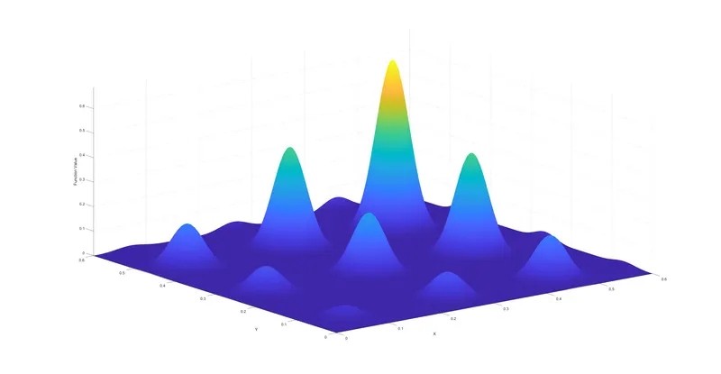
Figure 1-Stalagmite function

The matlab program to find maxima of given function is given below

clear all
close all
clc

% Defining function domain
x=linspace(0,0.6,150);
y=linspace(0,0.6,150);

% Setting number of iterations
num_cases=50;

% Evaluating stalagmite function
for i=1:length(x)
    for j=1:length(y)
        input_vector(1)=x(i);
        input_vector(2)=y(j);
        f(i,j)=stalagmite(input_vector);
    end
end

% Study 1-Statistical behavior
for n=1:num_cases
    [inputs, fval(n)]=ga(@stalagmite,2);
    xopt(n)=inputs(1);
    yopt(n)=inputs(2);
end
% Plotting unbounded statistical behaviour
figure(1)
subplot(2,1,1)
hold on
surfc(x,y,-f)
grid on
shading interp
view([-37.5 30])
xlabel('X')
ylabel('Y')
zlabel('Function Value')
plot3(xopt,yopt,-fval,'marker','o','markersize',5,'markerfacecolor','r')
title('Unbounded inputs')
subplot(2,1,2)
plot(-fval)
axis([1 inf 0 1])
xlabel('Iterations')
ylabel('Function maximum')

% Study 2-Statistical behavior with upper and lower bounds
for n=1:num_cases
    [inputs, fval(n)]=ga(@stalagmite,2,[],[],[],[],[0;0],[0.6;0.6]);
    xopt(n)=inputs(1);
    yopt(n)=inputs(2);
end
% Plotting statistical behaviour with upper and lower bounds
figure(2)
subplot(2,1,1)
hold on
surfc(x,y,-f)
grid on
shading interp
view([-37.5 30])
xlabel('X')
ylabel('Y')
zlabel('Function Value')
plot3(xopt,yopt,-fval,'marker','o','markersize',5,'markerfacecolor','r')
title('Bounded inputs')
subplot(2,1,2)
plot(-fval)
axis([1 inf 0 1])
xlabel('Iterations')
ylabel('Function maximum')

% Study 3-Increasing population size
% Using optimoptions to increase population size
options=optimoptions('ga');
options=optimoptions(options,'PopulationSize',170);
for n=1:num_cases
    [inputs, fval(n)]=ga(@stalagmite,2,[],[],[],[],[0;0],[0.6;0.6],[],[],options);
    xopt(n)=inputs(1);
    yopt(n)=inputs(2);
end

% Plotting statistical behavior with upper and lower bounds and increased
% population size
figure(3)
subplot(2,1,1)
hold on
surfc(x,y,-f)
grid on
shading interp
view([-37.5 30])
xlabel('X')
ylabel('Y')
zlabel('Function Value')
plot3(xopt,yopt,-fval,'marker','o','markersize',5,'markerfacecolor','r')
title('Bounded inputs with increased population size')
subplot(2,1,2)
plot(-fval)
axis([1 inf 0 1])
xlabel('Iterations')
ylabel('Function maximum')

% Determining maximum value of function and its coordinates
[max_val, max_ind]=max(-fval);
fprintf('\n The maximum value of function is %f at x=%f, y=%f\n',max_val,xopt(max_ind),yopt(max_ind))

The program can be divided into 4 parts. In the first part, the stalagmite function is evaluated by declaring its domain and substituting in function definition. This allows us to plot the function later. The second part consists of running ga function on stalagmite function without bounded search space. The third part consists of running ga function on stalagmite function with bounded search space. The fourth part consists of running ga function with bounded search space and increased population size. In all 3 cases, the ga function is run 50 times. In all 3 cases we get 50 values of x coordinate, y coordinate and function at maxima which are stored in xopt, yopt and fval respectively.

The program starts by clearing the workspace, command window and removing all plots. Then the domain of the function is specified with the help of linspace command. The values of both, x and y range from 0 to 0.6 over 150 values. The number of times ga function will be run in each study is declared next, which in this example is 50. The stalagmite function is then evaluated over its domain for various combinations of x and y coordinates. This is done by calling a function for stalagmite given below-

function [f]=stalagmite(input_vector)
    f1x=((sin((5.1*pi*input_vector(1))+0.5))^6);
    f2x=(exp(-4*log(2)*(((input_vector(1)-0.667)^2)/0.64)));
    f1y=((sin((5.1*pi*input_vector(2))+0.5))^6);
    f2y=(exp(-4*log(2)*(((input_vector(2)-0.667)^2)/0.64)));
    f=-f1x*f2x*f1y*f2y;
end

Stalagmite function requires the input of x coordinate and y coordinate in the form of a vector. The nested loop in the main program allows for the vector values to be assigned in a meshgrid like manner. For each value of x all 150 values of y are substituted in input vector one at a time, then the loop repeats for the next value of x until all x and y coordinates have been substituted in the function. In any given loop, the first value of vector is the x coordinate, and the second value of vector is the y coordinate at which function value is to be determined. Once values of function at each combination of cartesian coordinates has been determined, the function can be plotted using surfc command later in the program.

The next 3 parts are similar in structure. Most of each part is plotting the data generated in each for loop. Each for loop runs 50 times and differ based on the syntax of the ga function. As stated earlier, the ga function in the first study has an unbounded search space. The second and third study have a properly bound search space, but the third study has an increased population size over the second study.

Study 1-Unbound Search Space

for n=1:num_cases
    [inputs, fval(n)]=ga(@stalagmite,2);
    xopt(n)=inputs(1);
    yopt(n)=inputs(2);
end

In the given for loop ga function is used to find minima of function using unbound search space. This is because only the fitness function and number of variables have been specified in the syntax. The ga function returns the value of minima of function and a vector called ‘inputs’. The first element of this vector is the x coordinate of the predicted minima and the second element is the y coordinate of the predicted minima. The values of minima calculated and their coordinates for each of the 50 loops is stored in fval, xopt and yopt respectively.

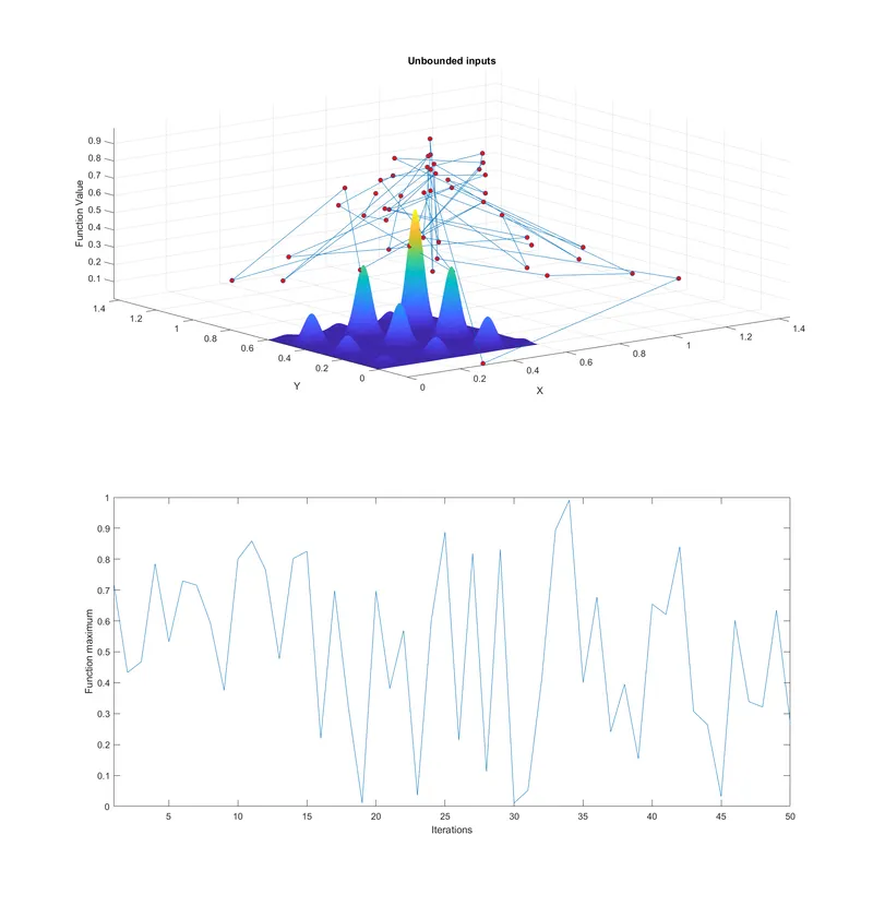
Figure 2-Statistical behaviour of GA function with unbounded search space

Figure 2 shows 2 subplots. The top subplot shows the function value over its domain overlayed with values of maxima predicted by ga function in each of the 50 iterations. This is done using surfc command and plot3 command, respectively. Hold on command is used to prevent overwriting data. Each value of maxima is plotted with a red circular marker and connected to the previous and next value of predicted maxima with a blue line. The lower subplot shows the value of function at maxima predicted versus the iteration number in which that maximum value was predicted. As the search space of ga function is unbound, it evaluates the function outside the function domain. This causes the predicted value at maxima to be erratic as can be seen from the lower subplot. The search space of ga function will be bound in study 2 and 3.

Study 2-Bound Search Space

for n=1:num_cases
    [inputs, fval(n)]=ga(@stalagmite,2,[],[],[],[],[0;0],[0.6;0.6]);
    xopt(n)=inputs(1);
    yopt(n)=inputs(2);
end

In this for loop, the syntax for ga function has been changed. The fitness function and number of variables are still the same, however the search space has been bound by the x and y coordinates, respectively. In the last 2 brackets of ga command the lower bound for x and y coordinate have been specified followed by upper value of x and y coordinate, respectively. This ensures that stalagmite function is only evaluated within its domain.

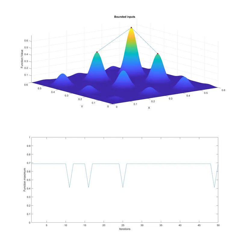
Figure 3-Statistical behaviour of GA function with bounded search space

Figure 3 shows that all 50 iterations converged to only 2 unique values of maxima, the global maxima and 2 local maxima. This also eliminates any possibility of predicting maxima values outside function domain. This greatly narrows down the results and eliminates the erratic behaviour in the first study. Only 4 iterations of for loop ended with maxima predicted at local maxima. The other 46 instances predicted the value and coordinates of global maxima correctly. To reduce the chance of predicting local maxima, the population of ga function can be increased, which is what is done in study 3.

Study 3- Bound Search Space and Increased Population

options=optimoptions('ga');
options=optimoptions(options,'PopulationSize',170);
for n=1:num_cases
    [inputs, fval(n)]=ga(@stalagmite,2,[],[],[],[],[0;0],[0.6;0.6],[],[],options);
    xopt(n)=inputs(1);
    yopt(n)=inputs(2);
end

Before the for loop begins, optimoptions function is used to change the population size of ga function. The optimoptions function allows user to change certain aspects of optimisation functions such as genetic algorithm. One of these aspects is population size. For any ga with less than 5 independent variables, the population size is taken as 50 by default. By manually increasing the population of initial guess to 170, the possibility of predicting local rather than global minima are reduced. This change is stored in the variable options and is used as an argument in ga function within the for loop.

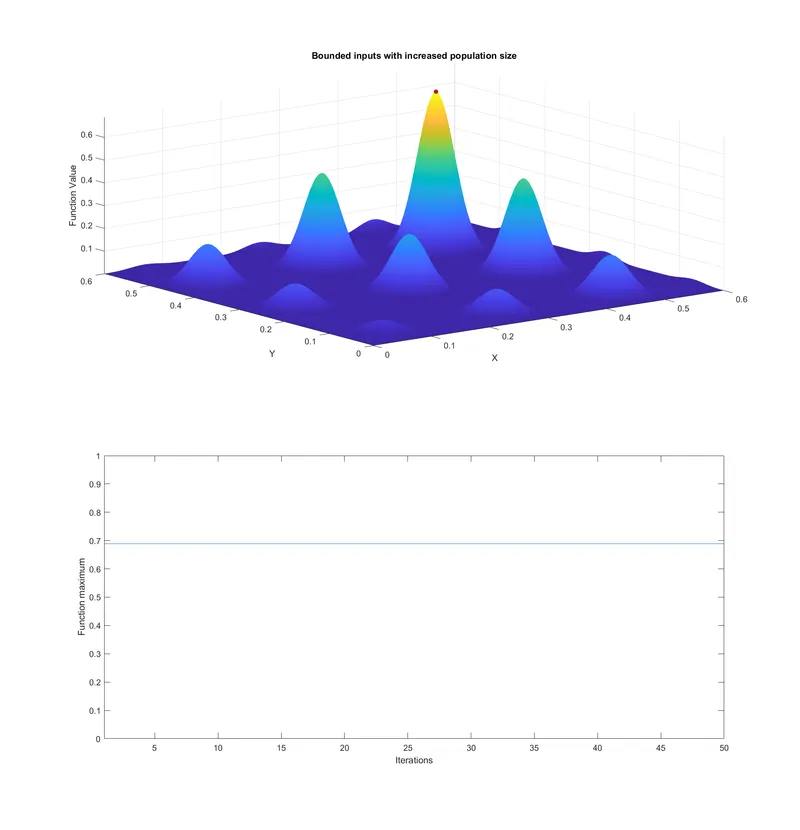
Figure 4-Statistical behaviour of GA function with bounded search space and increased population

Figure 4 shows us that all 50 iterations of for loop predict the same value of maxima. All 50 values are also the value of global maxima only and not local maxima. This is an excellent result as there are no outliers in the data points and function predicts global maxima accurately within function domain.

Detailed Description of Plotting

After each study, the data generated is plotted. The subplot command divides each figure window into 2 parts, one above the other. The hold on command is used to prevent overwriting of data. The stalagmite function is plotted along x and y axis using surfc command which generates a surface. The values of f are negative as the function is mirrored about x-y plane, since ga function can only calculate minima of function. Grid on command is used for easier viewing of data in top subplot. Shading interp varies the color at any point on the surface by interpolating the colormap index across the entire surface. The angle of viewing is set to -37.5 degrees of azimuth and 30 degrees of elevation for easy viewing of 3-dimensional data. The individual axes are labelled using xlabel, ylabel and zlabel. Zlabel being the value of function. Plot3 command is used to plot points in 3d space. This helps plot the x, y and z coordinate of each maxima predicted by ga function in each loop. The point is marked with a red circular marker and connected to the next and previous coordinates of maxima with blue lines. Finally, the title of the top subplot is written using the title command.

The next subplot is plotted with plot command. It generates a graph mapping the predicted value of maxima vs its corresponding iteration number. Again, the values of fval are negative as function is mirrored about x-y plane. The axis limits are set using axis command. This allows the range of graph to be fixed regardless of the range of values plotted. Finally, the horizontal axis is labelled as ‘Iterations’ and the vertical axis is labelled ‘Function maximum’.

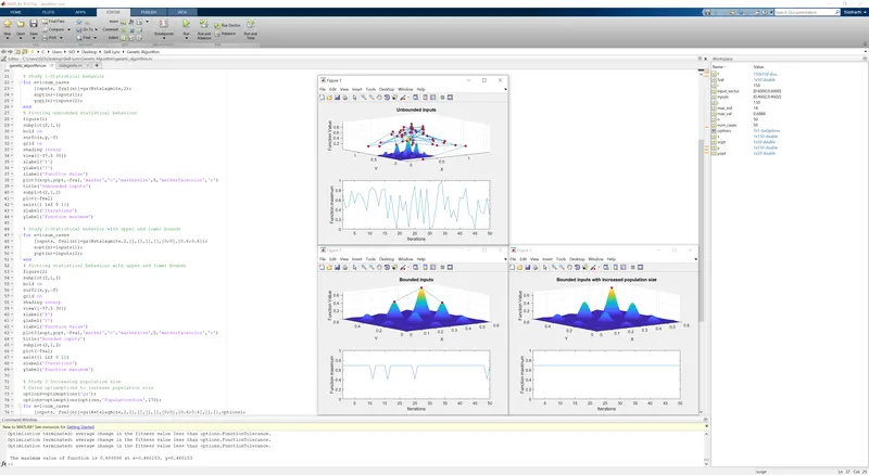
Figure 5-Test run of program

The final part of the program finds the maximum value of fval and its associated index numbers from study 3. Since function value, x coordinate and y coordinate are calculated in triples, xopt and yopt will have the same index value as the index of fval. The value of maxima and its coordinates are then printed using fprintf command.

CONCLUSION

The maximum value of function within its domain is 0.688806 at x=0.460153 and y=0.460153. This result is repeatable and does not vary from run to run.