Project 1 - Parsing NASA thermodynamic data
Parsing NASA Thermodynamic Data
AIM:
Write program that extracts 14 coefficients from output file and calculates enthalpy, entropy and specific heat for all species in data file.
OBJECTIVES:
- Calculate values of enthalpy, entropy and specific heat for all species using thermodynamic data from file.
- Plot the values of enthalpy, entropy and specific heat over the local temperature range of species.
- Save the plots as images in subfolders generated by the program.
- Calculate molecular weight of each species.
BODY OF WORK:
NASA has curve fit thermodynamic properties of various species using high order polynomials. The coefficients of these polynomials are listed in a file called THERMO.dat. The file contents need to be parsed, for the program to calculate thermodynamic properties of various species. The file contains a header given below-

Figure 1 - THERMO.dat Header
The header contains the name of the file on the first line, the global temperature values on the second line and some comments. The second value of the global temperature values denotes the temperature which marks the boundary between the low temperature range and high temperature range for calculating thermodynamic properties. The remainder of the file consists of blocks of 4 lines, each denoting properties of a particular species in scientific notation. An example is given below.

Figure 2 – Scientific Notation of Species Data in THERMO.dat
The block containing information about molecular oxygen is shown above. There are 80 columns and 4 rows in each block. This is important as the column number will be used for parsing data later in the program. The format of each block is explained below-
|
Row Number |
Contents |
Column Number |
|
1 |
Species Name |
1-18 |
|
1 |
Date (Optional) |
19-24 |
|
1 |
Atomic Symbols and Formula |
25-44 |
|
1 |
Phase of species (S, L, G) |
45 |
|
1 |
Species Low Temperature |
46-55 |
|
1 |
Species High Temperature |
56-65 |
|
1 |
Common Temperature |
66-73 |
|
1 |
Additional Atomic Symbols |
74-78 |
|
1 |
The integer 1 |
80 |
|
2 |
Coefficients a1 to a5 for high temperature interval |
1-75 |
|
2 |
The integer 2 |
80 |
|
3 |
Coefficients a6 and a7 for high temperature interval and coefficients a1 to a3 for the low temperature interval |
1-75 |
|
3 |
The integer 3 |
80 |
|
4 |
Coefficients a4 to a7 for the low temperature interval |
1-60 |
|
4 |
The integer 4 |
80 |
Table 1- Format of Thermodynamic Data of Species from THERMO.dat
The coefficients above are used to calculate the value of specific heat capacity, enthalpy and entropy of each species using the following formulae-
Specific heat capacity-
`cp=R*(a_1+(a_2*T)+(a_3*T^2 )+(a_4*T^3 )+(a_5*T^4 ))`
Enthalpy-
`h=R*((a_1*T)+(a_2*T^2/2)+(a_3*T^3/3)+(a_4*T^4/4)+(a_5*T^5/5)+a_6)`
Entropy-
`s=R*((a_1*ln(T))+(a_2*T)+(a_3*T^2)+(a_4*T^3)+(a_5*T^4)+a_7)`
The formulae have a temperature domain divided into two parts. The low temperature interval and the high temperature interval. The formulae change definition at 1000 K. The Low temperature interval of each species extends from the species low temperature to 1000 K. The high temperature interval of each species extends from 1000 K to the species high temperature.
The program is written in matlab and is given below
clear all
close all
clc

f1=fopen('THERMO.dat','r');
R=8.314;

% Header
fgetl(f1);
A=strsplit(fgetl(f1),' ');
global_low_temp=str2num(A{2});
global_mid_temp=str2num(A{3});
global_high_temp=str2num(A{4});
fgetl(f1);
fgetl(f1);
fgetl(f1);

for i=1:53
    % Line #1
    tline=fgetl(f1);
    name=strtok(tline);
    min_temp=str2num(tline(49:55));
    max_temp=str2num(tline(58:65));
    T=linspace(min_temp,max_temp,500);
    mol_w=0;
    for j=1:4
        c=25+(5*(j-1));
        d=c+4;
        if tline(c)=='C'
            mol_w=mol_w+(12.0107*str2num(tline(d)));
        elseif tline(c)=='H'
            mol_w=mol_w+(1.00784*str2num(tline(d)));
        elseif tline(c)=='O'
            mol_w=mol_w+(15.999*str2num(tline(d)));
        elseif tline(c)=='N'
            mol_w=mol_w+(14.0067*str2num(tline(d)));
        elseif (tline(c)=='A')&&(tline(c+1)=='R')
            mol_w=mol_w+39.948;
        else
            mol_w=mol_w+0;
        end
    end
    j=0;
    fprintf('molecular weight of %s=%f\n',name,mol_w)

    % Line #2
    tline=fgetl(f1);
    k=findstr(tline,'E');
    a1=tline(1:k(1)+3);
    a1=str2num(a1);
    a2=tline(k(1)+4:k(2)+3);
    a2=str2num(a2);
    a3=tline(k(2)+4:k(3)+3);
    a3=str2num(a3);
    a4=tline(k(3)+4:k(4)+3);
    a4=str2num(a4);
    a5=tline(k(4)+4:k(5)+3);
    a5=str2num(a5);

    % Line #3
    tline=fgetl(f1);
    l=findstr(tline,'E');
    a6=tline(1:l(1)+3);
    a6=str2num(a6);
    a7=tline(l(1)+4:l(2)+3);
    a7=str2num(a7);
    a8=tline(l(2)+4:l(3)+3);
    a8=str2num(a8);
    a9=tline(l(3)+4:l(4)+3);
    a9=str2num(a9);
    a10=tline(l(4)+4:l(5)+3);
    a10=str2num(a10);

    % Line #4
    tline=fgetl(f1);
    m=findstr(tline,'E');
    a11=tline(1:m(1)+3);
    a11=str2num(a11);
    a12=tline(m(1)+4:m(2)+3);
    a12=str2num(a12);
    a13=tline(m(2)+4:m(3)+3);
    a13=str2num(a13);
    a14=tline(m(3)+4:m(4)+3);
    a14=str2num(a14);

    % Calling functions
    cp=sp_heat(a1,a2,a3,a4,a5,a8,a9,a10,a11,a12,T,global_mid_temp,R);
    h=enthalpy(a1,a2,a3,a4,a5,a6,a8,a9,a10,a11,a12,a13,T,global_mid_temp,R);
    s=entropy(a1,a2,a3,a4,a5,a7,a8,a9,a10,a11,a12,a14,T,global_mid_temp,R);

    % Create subfolder if it doesn't exist
    if ~exist(name,'dir')
        mkdir(name)
    end

    % change directory to subfolder
    cd(name)

    % Plot specific heat capacity vs temperature
    figure('Name',name,'visible','off')
    title(sprintf('Specific heat capacity vs Temperature of %s',name))
    hold on
    plot(T,cp);
    xlabel('Temperature (K)')
    ylabel('Specific heat capacity (J/mol-K)')
    grid on
    saveas(gcf,'specific heat capacity.png')

    % Plot enthalpy vs temperature
    figure('Name',name,'visible','off')
    title(sprintf('Enthalpy vs Temperature of %s',name))
    hold on
    plot(T,h);
    xlabel('Temperature (K)')
    ylabel('Enthalpy (J/mol)')
    grid on
    saveas(gcf,'enthalpy.png')

    % Plot entropy vs temperature
    figure('Name',name,'visible','off')
    title(sprintf('Standard Entropy vs Temperature of %s',name))
    hold on
    plot(T,s);
    xlabel('Temperature (K)')
    ylabel('Standard Entropy (J/mol-K)')
    grid on
    saveas(gcf,'entropy.png')

    % Change directory to parent folder
    cd('..')
end
The program starts by clearing the workspace, command window and removing all plots. The “fopen” command is used to open the file for binary read access and the integer file identifier is stored in variable “f1”. This will be used as pointer for the remainder of the program. The gas constant R is specified next as 8.314 J/mol-K. The header file is then parsed for data. The “fgetl” command returns the first line of the file THERMO.dat. As this contains only the word “THERMO” it is of no use for calculating thermodynamic values. The “fgetl” command is used again to move to the next line and return the values in the form of a string. This line contains the global temperature values. The string is split using “strsplit” command which scans the line for the user specified character “ ”, blank space. Thus the second line of file THERMO.dat is divided into a 1x4 cell array and which is stored in variable “A”. The “str2num” command is used to convert strings to numbers. The second, third and fourth parts of the cell “A” contain the values of global low temperature, global common temperature, and global high temperature. The “str2num” command is used on array “A” to store each value in a variable named accordingly. The next three lines are comments which are also not useful for calculating thermodynamic data and the “fgetl” command is used 3 times to scan the three lines only to get to the last line of the header.
Now that all the rest of the blocks have a common format, a loop can be used to scan through each one line by line. A for loop is started for all 53 species. The “fgetl” command is used for used for storing the first line as a string in the variable “tline”. The command “strtok” splits the string using the position of blank spaces and returns the first piece of that string to the assigned variable. The “strtok” command is thus used for saving the species name to the variable “name” in the form of a string. The “str2num” command is used to scan and convert the characters in column 49 to 55 and store them as a number in variable “min_temp”. This specifies the lower limit of temperature of low temperature interval for the given species. The “str2num” command is then used to scan and convert the characters in column 58 to 65 and store them as a number in variable “max temp”. This specifies the upper limit of temperature of high temperature interval. The “linspace” command is then used to divide the range of temperature between the upper and lower limits into 500 parts and store them in variable “T”. The values in array “T” will be substituted in formulae to calculate the values of entropy, enthalpy and specific heat capacity later in the program. A variable “mol_w” is declared and will be used to store and print the value of molecular weight of each species. Column number 25 to 44 are used to store the number of atoms of each type in 4 blocks. The first character of each block contains the symbol of the constituting atom. The last character of each block contains the number of atoms of that type constituting the species. This means that each species can only be constituted by up to 4 types of atoms. A for loop to scan all 4 blocks is started. The column number of the first element of the block is stored in variable “c” and the column number of the last element of the block is stored in variable “d”. If the element in column number “c” is “C”,“H”,“O” or “N” the variable for molecular weight is incremented by the product of atomic mass of carbon, hydrogen, oxygen or nitrogen and the corresponding number of atoms constituting the species. The only exception to this is argon. It is the only species in THERMO.dat that’s atomic name consists of 2 characters. A separate condition is written which increments the value of molecular weight by the atomic mass of argon. Once all 4 blocks have been scanned and the molecular weight of species has been calculated the program prints the value of molecular weight of the current species in the command window using the “fprintf” command.
The next 3 lines of THERMO.dat are parsed in the same way. The “fgetl” command is used to move to the next line and store the value of the string in variable “tline”. The “findstr” command is used to find the user specified character “E” in the string. It also stores an array with all the column numbers containing character “E” in the variable “k”. The base of the coefficient occupies 11 columns preceding the character “E” in every coefficient. The exponent of the coefficient occupies 3 columns following the character “E” in every coefficient. Keeping this in mind, variables a1 to a14 store the values of the corresponding coefficient as a string. Then these variables are overwritten to store the values of coefficient as a number using “str2num” command. Using this method we obtain the values of 5 coefficients from line #2, 5 coefficients from line #3 and 3 coefficients from line #4.
The values of temperature calculated earlier using “linspace” command, 14 coefficients and the value of gas constant are substituted in 3 functions. These 3 functions calculate the value of specific heat capacity, enthalpy and entropy respectively. The functions are given below-
Specific heat capacity
function [cp]=sp_heat(a1,a2,a3,a4,a5,a8,a9,a10,a11,a12,T,global_mid_temp,R)
    if T<=global_mid_temp
        cp=R*(a8+(a9.*T)+(a10.*(T.^2))+(a11.*(T.^3))+(a12.*(T.^4)));
    else
        cp=R*(a1+(a2.*T)+(a3.*(T.^2))+(a4.*(T.^3))+(a5.*(T.^4)));
    end
end
Enthalpy
function [h]=enthalpy(a1,a2,a3,a4,a5,a6,a8,a9,a10,a11,a12,a13,T,global_mid_temp,R)
    if T<=global_mid_temp
        h=R*((a8.*T)+((a9.*(T.^2))./2)+((a10.*(T.^3))./3)+((a11.*(T.^4))./4)+((a12.*(T.^5))./5)+a13);
    else
        h=R*((a1.*T)+((a2.*(T.^2))./2)+((a3.*(T.^3))./3)+((a4.*(T.^4))./4)+((a5.*(T.^5))./5)+a6);
    end
end
Entropy
function [s]=entropy(a1,a2,a3,a4,a5,a7,a8,a9,a10,a11,a12,a14,T,global_mid_temp,R)
    if T<=global_mid_temp
        s=R*((a8.*log(T))+(a9.*T)+(a10.*(T.^2))+(a11.*(T.^3))+(a12.*(T.^4))+a14);
    else
        s=R*((a1.*log(T))+(a2.*T)+(a3.*(T.^2))+(a4.*(T.^3))+(a5.*(T.^4))+a7);
    end
end
These functions change their definition based on the substituted value of temperature. If “T” is part of the high temperature interval, the first set of 7 coefficients are used. If “T” is part of the low temperature interval, the second set of 7 coefficients are used.
Before creating plots for the data generated, we must check if a subfolder with the species name exists in current directory using “~exist” command. If not, then the subfolder is created using “mkdir” command and assigned the name of the species. The “cd” command changes the directory to the subfolder with name of species. Now that we are in the correct subfolder, plots can be generated and saved.
The three graphs to be plotted are specific heat capacity vs temperature, enthalpy vs temperature and entropy vs temperature. Three blocks of code, using the same structure are used to plot and save data. The first line of each block creates a new figure. The name of each figure is the species name. Since the plot will be saved in the subfolder later, the visibility of the figure is turned off. The second line prints the title of the plot, giving each plot an appropriate description and name of species. The third line contains the “hold on” command which prevents overwriting of data while plotting. The fourth line plots the values of temperature and corresponding values of thermodynamic property calculated by functions earlier. Values of specific heat capacity, enthalpy and entropy are plotted on the vertical axis and take their values from array “cp”, “h” and “s” respectively. Temperature is plotted on the horizontal axis for all values ranging from species low temperature to species high temperature. The fifth line labels the horizontal axis as temperature in kelvin using the “xlabel” command. The sixth line labels the vertical axis as the thermodynamic property being plotted using the “ylabel” command. The seventh line superimposes a grid on the plot for easier viewing. The last line saves the plotted graph as .png file using figure handle “gcf” and file name provided in single quotes. Once all three plots for a given species are saved to the subfolder named after the species, the “cd” command is used again to change directory to the parent folder. After this the for loop repeats for the next species until all 53 values of molecular weight have been calculated and all 159 plots have been saved.
CONCLUSION:

Figure 3 – Screenshot of All Folders
Thermodynamic properties and molecular weight of all species have been calculated. A screenshot of the molecular weights in command window of matlab is shown below.
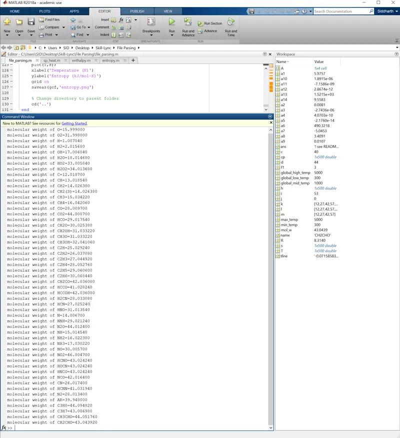
Figure 4 – Molecular weight of All Species
The plots for species O2, N2 and CO2 are shown below.
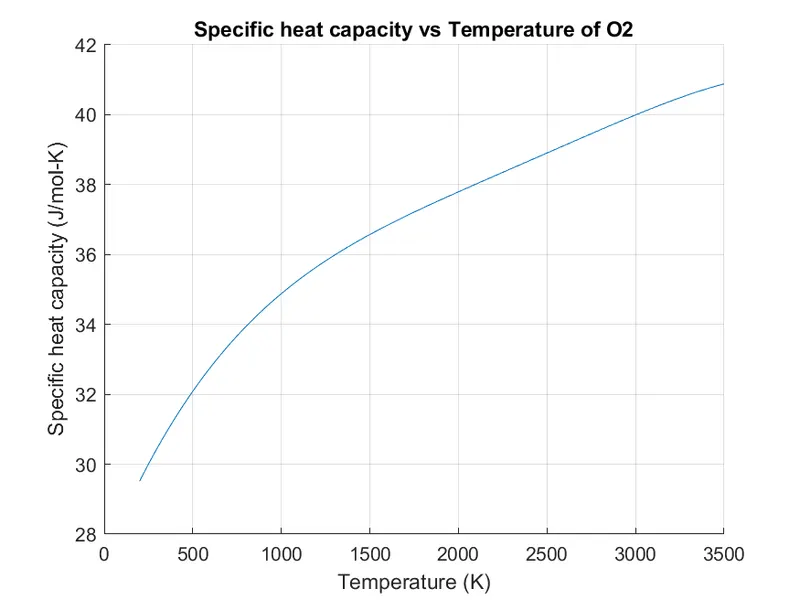
Figure 5 – Specific Heat Capacity vs Temperature of O2
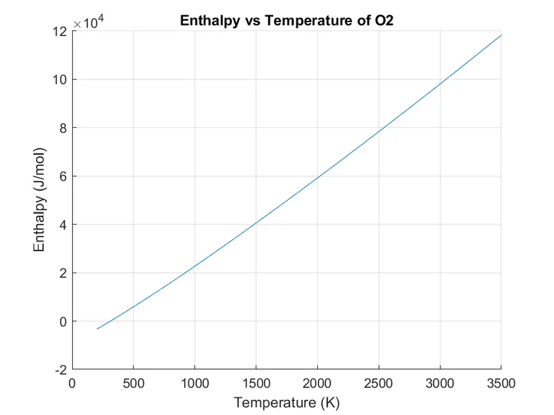
Figure 6 – Enthalpy vs Temperature of O2
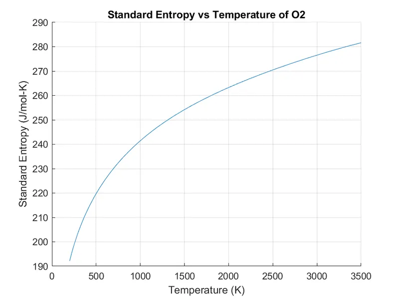
Figure 7 – Entropy vs Temperature of O2
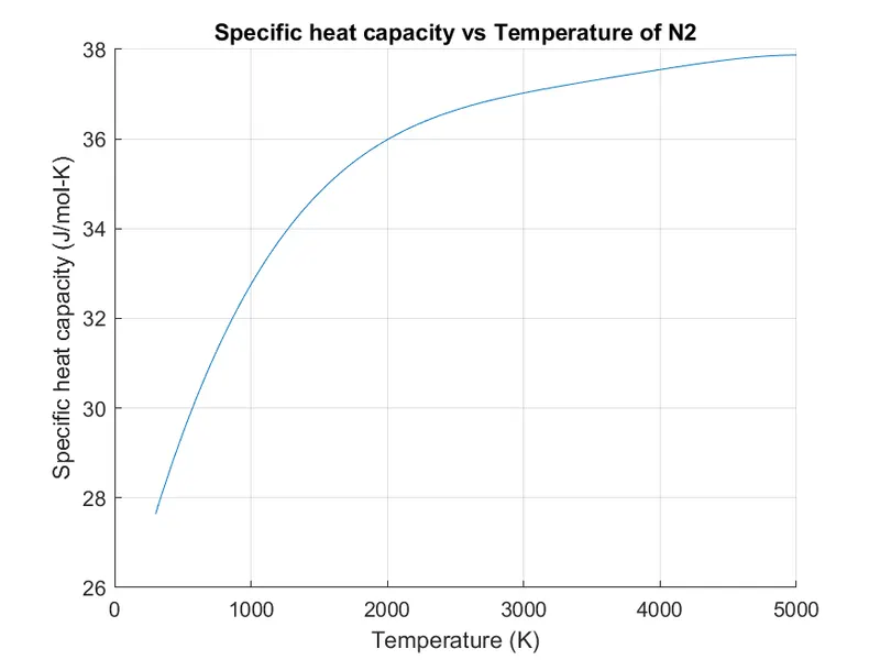
Figure 8 – Specific Heat Capacity vs Temperature of N2
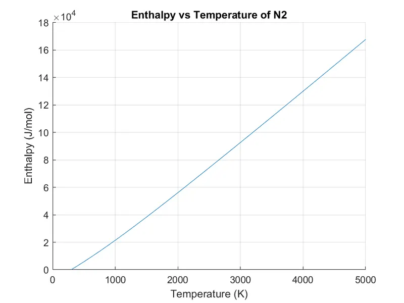
Figure 9 – Enthalpy vs Temperature of N2
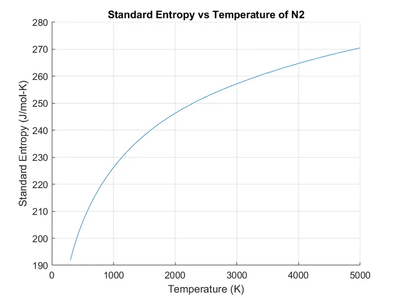
Figure 10 – Entropy vs Temperature of N2
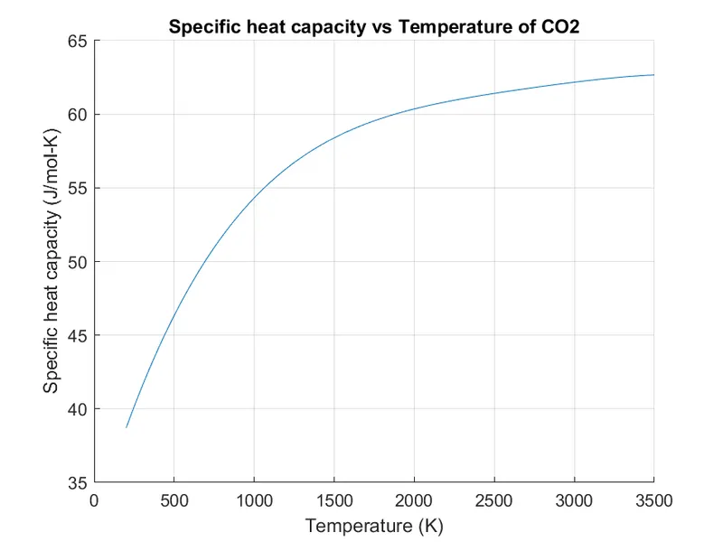
Figure 11 – Specific Heat Capacity vs Temperature of CO2
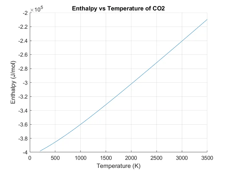
Figure 12 – Enthalpy vs Temperature of CO2
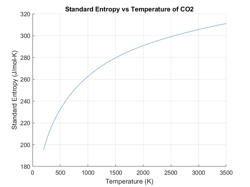
Figure 13 – Entropy vs Temperature of CO2
REFERENCES:
https://cantera.org/tutorials/ck2cti-tutorial.html