Week 3 - Solving second order ODEs

Second Order Ordinary Differential Equation

AIM: Write Matlab program to simulate damped vibration.

OBJECTIVE: Solve second order ordinary differential equation to simulate movement of pendulum and create video of it.

BODY OF CONTENT:

Motion of pendulum is given by following second order ordinary differential equation-

`(d^2 θ)/(dt^2) +b/m (dθ)/dt+g/L sinθ=0`

Where

g=gravitational acceleration

L=length of pendulum

m=mass of the pendulum

b=damping coefficient

Matlab has an inbuilt function which helps us solve differential equations but to solve second order differential equation we need to substitute in above equation to get two separate first order differential equations. Thus, we make the following substitutions in above formula-

`θ=θ_1`

`(dθ_1)/dt=θ_2`

Substituting both above equations in first equation we get

`(dθ_2)/dt+b/m θ_2+g/L sinθ_1=0`

Changing the subject of formula, we get

`(dθ_2)/dt=-b/m θ_2-g/L sinθ_1`

Rewriting above in matrix form we get-

`d/dt [(θ_1@θ_2 )]=[(θ_2@-b/m θ_2-g/L sinθ_1 )]`

This equation is used to solve for the position and velocity of the pendulum at every point on its traverse. The variables are given the following values-

g=9.81 m/s²

L=1 m

m=1 kg

b=0.05

On solving the first equation using these values the solution for the first 20 seconds of pendulum motion looks like-

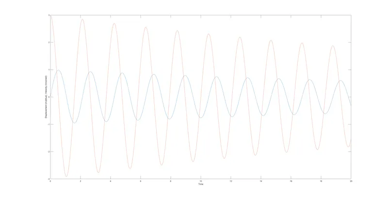
Figure 1- Pendulum displacement (m)(blue) and Pendulum velocity (m/s²)(red) vs time

Program is written in Matlab and is attached below.

clear all
close all
clc

b=0.05;
g=9.81;
l=1;
m=1;

% initial condition [angular displacement;velocity]
theta_0=[0;3];

% time span
t_span=linspace(0,20,101);

% solve ODE
[t, results]=ode45(@(t,theta) ode_func(t,theta,b,g,l,m),t_span,theta_0);

% plotting
results(:,1)=results(:,1)+(1.5*pi);
x0=0;
y0=1;
for i=1:101
    x1=l*cos(results(i,1));
    y1=y0+l*sin(results(i,1));
    plot([x1],[y1],'bo','MarkerSize',40,'markerfacecolor','b')
    hold on
    plot([x0 x1],[y0 y1],'b','linewidth',3)
    hold off
    axis([-1 1 0 1])
    xlabel('Horizontal Displacement (m)')
    ylabel('Vertical Displacement (m)')
    M(i)=getframe(gcf);
    i=i+1;
end

movie(M)
videofile=VideoWriter('pendulum.avi','Uncompressed AVI');
open(videofile)
writeVideo(videofile,M)
close(videofile)

Program uses user specified data to simulate motion of pendulum undergoing damped vibration. The program starts by clearing the workspace, command window and removing all plots. User then inputs values of gravitational acceleration, length of pendulum, mass of pendulum and damping coefficient. Then the initial conditions of pendulum are specified by user. Here we have assigned the motion of pendulum to start at zero displacement from the vertical and at a speed of 3 m/s. The final input before proceeding to solve is the time span for which we simulate the motion of pendulum oscillation. Here we have used the linspace command to specify that the simulation will begin at 0 seconds and end at 20 seconds with 101 intervals of time in between so that each time interval is exactly 0.2 seconds.

Next, we use the matlab function ode45 to solve our ordinary differential equation. To do that we specify that ordinary differential equation is a function of time(t) and pendulum angle(theta). Then we define our function which is named ode_func and uses the variables t, theta, b, g, l and m. Then we specify the values of t which will be substituted in function definition. This is given by t_span ranging from 0 to 20 in 0.2 second increments to form an array of 101 elements. Finally, user specifies the initial conditions of velocity and displacement at the beginning of simulation using theta_0.

Function is defined as follows

function[dtheta_dt]=ode_func(t,theta,b,g,l,m)
    theta1=theta(1);
    theta2=theta(2);
    dtheta1_dt=theta2;
    dtheta2_dt=-(b/m)*theta2-(g/l)*sin(theta1);
    dtheta_dt=[dtheta1_dt; dtheta2_dt];
end

Here we solve the matrix equation calculated earlier for every value of time specified by t_span. Thus for every value of time we get a corresponding value of angular displacement(theta1) and velocity of pendulum(theta2). The function uses b, g, l, m, t, and initial values of displacement and velocity to create a two-column matrix of values. These two columns contain the calculated values of theta1 and theta 2 and are passed back to the main program where they are stored in a matrix called results. The first column of results matrix contains values of theta1 and the second column contains values of theta2. This matrix will be used to plot animation

As the pendulum swings downwards and angular displacement is measured from the vertical, 270 degrees is added to all the values of theta1 which is given in radians. The initial coordinates of the free end of the pendulum are specified at origin with its fixed end, 1m above origin. To plot the location of the pendulum, the coordinates of the free end of pendulum must be calculated. To plot values of x1 and y1 a loop must be used as x1 and y1 keep changing with time.

A for loop is started which increments 101 times, once for each value of time. Within each loop a unique value of x1 and y1 are calculated, plotted, stored, and then overwritten in the next loop. The values of x1 and y1 are calculated using trigonometry, since we know the angle and length of pendulum. The pendulum bob is plotted first using marker command. The coordinates of the pendulum are given by x1 and y1. The marker color and shape are selected as a blue circle. Marker size is selected using markersize and is colored solid blue using markerfacecolor. Then for each position of pendulum a line joining fixed and free end of pendulum is drawn in blue using plot command. Hold on and hold off command are used to prevent overwriting of plots within a loop and allow plots to be overwritten once next loop begins. Extent of displayed space for plotting is specified using axis command. Here, only space up to 1m above horizontal axis is displayed as pendulum does not swing past 90 degrees, nor does its length allow it to extend below horizontal axis. The horizontal axis is labelled as horizontal displacement and the vertical axis is labelled as vertical displacement of the pendulum weight, using xlabel and ylabel commands. Within each loop, a position of pendulum is plotted and stored in array M using getframe command. Each frame stored in array M is used to create a video file. Before ending loop, the count variable i is incremented.

Now that plots are stored in array M, they are written frame by frame to uncompressed video file pendulum.avi using VideoWriter command. The file must be named, opened, written to using array M, and then closed. This allows the individual plots to be saved as a video outside matlab program.

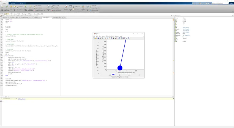
Figure 2-Program Output

Shown above is the matlab program running. In the middle is the last captured frame of the animation. The horizontal axis shows the displacement of pendulum weight from center. The vertical axis shows the displacement of pendulum weight above its lowest position at origin. As described previously, t is an array of 101 values as is t_span. On the other hand results is a 101*2 matrix as it contains values of both angular displacement as well as velocity of pendulum for each value of t.

CONCLUSION

Program correctly simulates damped vibrations of pendulum and creates video file of pendulum motion. To access the video, follow the given link https://youtu.be/fH3Ln6FcScc

One possible improvement that can be made in accordance with the animation in the question, is to display the velocity of pendulum weight as well as position. The following matlab program displays the direction and magnitude of velocity as a red line in addition to the position of pendulum.

clear all
close all
clc

b=0.05;
g=9.81;
l=1;
m=1;

% initial condition [angular displacement;velocity]
theta_0=[0;3];

% time span
t_span=linspace(0,20,101);

% solve ODE
[t, results]=ode45(@(t,theta) ode_func(t,theta,b,g,l,m),t_span,theta_0);

% plotting
results(:,3)=results(:,1)+(1.5*pi);
x0=0;
y0=1;
for i=1:101
    x1=l*cos(results(i,3));
    y1=y0+l*sin(results(i,3));
    x2=x1+(results(i,2))*cos(results(i,1));
    y2=y1+(results(i,2))*sin(results(i,1));
    plot([x1],[y1],'bo','MarkerSize',40,'markerfacecolor','b')
    hold on
    plot([x0 x1],[y0 y1],'b','linewidth',3)
    plot([x1 x2],[y1 y2],'r','linewidth',3)
    hold off
    axis([-3 3 -1 2])
    xlabel('Horizontal Displacement (m)')
    ylabel('Vertical Displacement (m)')    
    M(i)=getframe(gcf);
    i=i+1;
end

movie(M)
videofile=VideoWriter('pendulum_alt.avi','Uncompressed AVI');
open(videofile)
writeVideo(videofile,M)
close(videofile)