Simulation of ideal Otto Cycle

Simulation of Ideal Otto Cycle

AIM: Write Matlab program to simulate ideal otto cycle.

OBJECTIVE:

Write a program which plots pressure-volume diagram of ideal otto cycle and calculates thermal efficiency.

BODY OF CONTENT: Program is written in Matlab and is attached below.

clear all
close all
clc

%Inputs
gamma=1.4;
t3=2300;

%State Variables
p1=101325;
t1=500;

%Engine Geometric Parameters
bore=0.1;
stroke=0.1;
con_rod=0.15;
cr=12;

%Calculating Swept Volume
v_s=pi/4*bore^2*stroke;

%Calculating Clearance Volume
v_c=v_s/(cr-1);

%Volume at bottom dead centre
v1=v_c+v_s;

%Volume at top dead centre
v2=v_c;

%Calling function
V_expansion=engine_kinematics(stroke,con_rod,cr,v_c);
V_compression=flip(V_expansion);

%State variables at state point 2
%For isentropic process
%p2v2^gamma=p1v1^gamma
%p2=p1*(v1/v2^gamma)=p1*cr^gamma
p2=p1*cr^gamma;
P_compression=(p1*v1^gamma)./V_compression.^gamma;

%Using ideal gas law
%p1v1/t1=p2v2/t2
t2=p2*v2*t1/(p1*v1);

%State variables at state point 3
v3=v2;

%Using ideal gas law
%p3v3/t3=p2v2/t2
p3=p2*t3/t2;

%State variables at state point 4
v4=v1;
%For isentropic process
%p3v3^gamma=p4v4^gamma
p4=p3*(v3/v4)^gamma;
P_expansion=(p3*v3^gamma)./V_expansion.^gamma;

%Using ideal gas law
%p4v4/t4=p3v3/t3
t4=p4*v4*t3/(p3*v3);

%Efficiency calculation
%efficiency=1-(1/(cr^(gamma-1)))
efficiency=1-(cr^(1-gamma))

figure(1)
hold on
plot(V_compression, P_compression)
plot([v2 v3], [p2 p3])
plot(V_expansion, P_expansion)
plot([v4 v1], [p4 p1])
xlabel('Volume (m^3)')
ylabel('Pressure (Pa)')

Program uses user specified data to simulate ideal otto cycle in single cylinder engine. Intake and exhaust stroke are not shown as they are a horizontal line from state 1, parallel to the x-axis and contribute no work to the cycle. Instead, this program concentrates on the compression and power strokes.

The first state is given at the end of the intake stroke, when the piston is at bottom dead center and is at atmospheric pressure. From here, the air inside the cylinder undergoes isentropic compression to reach state 2. From state 2, ignition of charge causes constant volume heat addition to reach state 3. From state 3, charge undergoes isentropic expansion to reach state 4. From state 4, exhaust is assumed to evacuate cylinder instantaneously using constant volume heat rejection, to return to state 1.

The program starts by clearing the workspace, command window and removing all plots. User provides data for ratio of specific heats, given by gamma and temperature of charge after ignition, as program does not simulate chemical kinetics. The user then specifies pressure and temperature at state 1. Finally, the user specifies geometric dimensions of engine, namely bore, stroke, connecting rod length and compression ratio.

Using the formula for volume of cylinder, the swept volume of cylinder is calculated. The clearance volume is then calculated using the relation

Clearance Volume=Swept Volume/(Compression Ratio-1)

The volume of cylinder at state 1 is then calculated as the sum of clearance volume and swept volume, giving us volume at bottom dead center. The volume at state 2 is also calculated, as the clearance volume is equal to the volume at top dead center.

A function is then called. The function is given below.

function [V]=engine_kinematics(stroke,con_rod,cr,v_c)
    R=con_rod*2/stroke;
    theta=linspace(0,180,180);
    V=(1+(0.5*(cr-1))*((R+1-cosd(theta))-((R^2-sind(theta).^2).^0.5))).*v_c;
end

This function uses stroke, connecting rod length, compression ratio and clearance volume to calculate an array of variables. This array contains values of the volume of cylinder for each degree of crank rotation for 180 degrees. To calculate this array, another variable called rod ratio is calculated by dividing connecting rod length by crank pin offset.

In this instance, function is used to calculate the volume of cylinder for each crank angle from top dead center to bottom dead center and store the values of volume in an array called V. This array of variables is then passed to the main program and stored as an array called V_expansion. During the compression process the cylinder again undergoes the same change of volume, only from bottom dead center to top dead center. Thus, to obtain the array for V_compression, the order of elements in V_expansion is reversed using flip command.

Now that pressure, temperature, and volume at state 1 are known we can calculate the same for state 2. Volume at state 2 is already known to be clearance volume. For isentropic process, the following formula holds true

p₁v₁^γ=p₂v₂^γ

By rearranging and substituting for compression ratio in this formula we find the value of p2 which is equal to p₁*(compression ratio)^γ. As the isentropic compression process cannot be denoted by a straight line between state 1 and 2 on a pressure-volume diagram, we must plot multiple values of pressure and volume to plot the correct curve. Since we have an array of values of volume, we can use the V_compression array to calculate an array for storing values of pressure. P_compression array is calculated in the same way as p2 was, the only difference being that the element wise operator is used to operate on each element one at a time.

Once p2 and P_compression have been calculated we can use the ideal gas law to calculate temperature at state 2. The ideal gas law states that

p₁v₁/t₁= p₂v₂/t₂

On rearranging and making t2 as subject we get the value of t2 as p₂*v₂*t₁/(p₁*v₁). Thus, values of pressure, temperature and volume at state 2 have been calculated as well as pressure and volume array for isentropic compression process.

Volume at state 3 is the same as state 2 as heat addition is done at constant volume. Hence, v₃=v₂. Temperature at state 3 is given by user as t₃ cannot be calculated without chemical kinetics which is out of the scope of this program. Now that temperature and volume at state 3 are known, ideal gas law is used to calculate pressure at state 3.

Volume at state 4 is the same as state 1 as they are both at bottom dead centre. Thus v₄=v₁. Just like in isentropic compression, pressure at state 4 is calculated by making p₄ the subject of the following equation and solving

p₃v₃^γ=p₄v₄^γ

Just like in the isentropic compression process we can use the V_expansion array to calculate values of P_expansion using element wise operator, seeing as p₃v₃^γ is constant throughout the process. Finally, the temperature at state 4 is calculated using ideal gas law given as follows

p₄v₄/t₄= p₃v₃/t₃

By making t₄ subject we can solve for temperature at state 4. Now temperature, pressure and volume at each of the 4 states has been calculated.

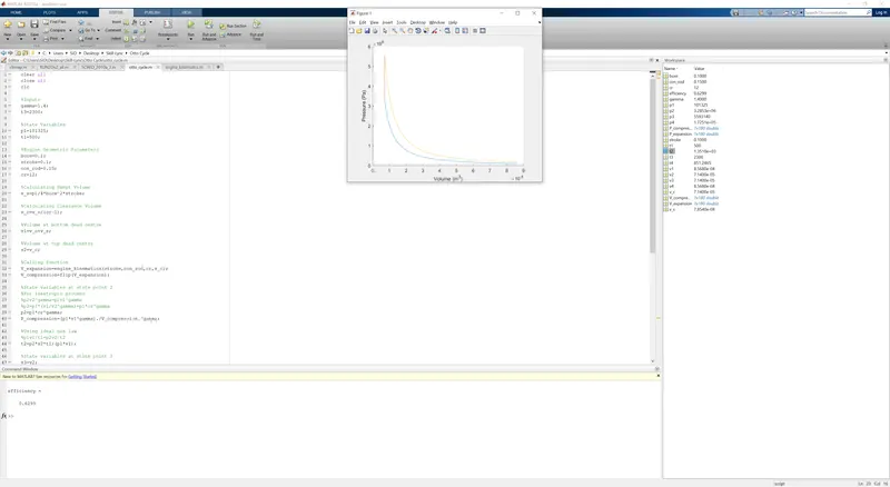
Figure 1-Test run

The final step before plotting is to calculate cycle efficiency which is given by the following formula

Efficiency=1-Compression Ratio^(1-gamma)

Finally, the pressure volume diagram of the otto cycle is plotted. Isochoric processes 2-3 and 4-1 are denoted by straight vertical lines. The isentropic compression process is plotted using V_compression and P_compression arrays. The isentropic expansion process is plotted using V_expansion and P_expansion arrays. All four arrays have 180 elements each. Plots are made with hold on command so that they are not overwritten. The x-axis is labeled volume in cubic meters and the y-axis is labeled pressure in pascal.

CONCLUSION

The Pressure Volume graph is plotted as follows

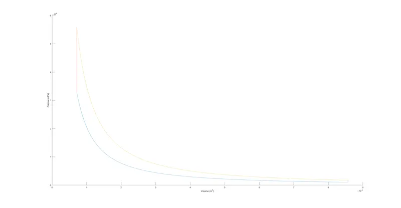
Figure 2- Pressure-Volume diagram of Otto cycle

Blue Line-Isentropic Compression from state 1 to state 2

Red Line-Constant volume heat addition from state 2 to state 3

Yellow Line-Isentropic expansion from state 3 to state 4

Purple Line-Constant volume heat rejection from state 4 to state 1

The efficiency of the cycle for the given conditions is calculated to be 0.6299 or roughly 63%.

Link for report on project page is https://skill-lync.com/projects/simulation-of-ideal-otto-cycle